Fixed-time prescribed performance formation control of heterogeneous UAV-USV systems under actuator faults

2.1. USV model

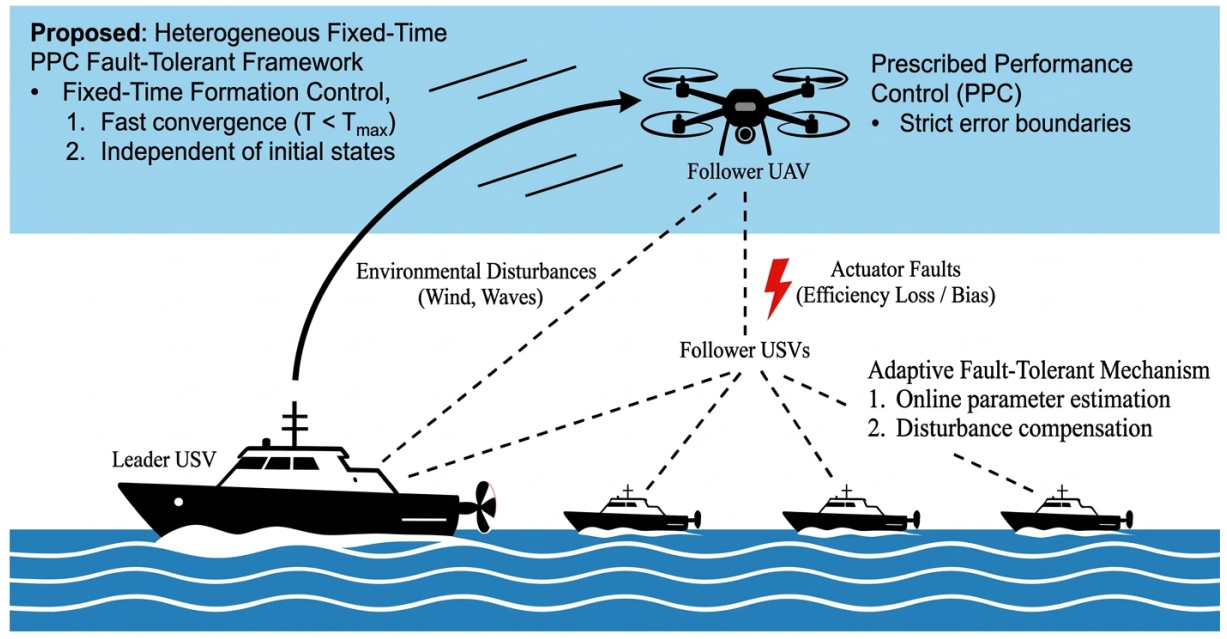
Consider a heterogeneous system consisting of one leader USV, multiple follower USVs, and one follower UAV. The coordinate systems of the heterogeneous UAV-USV cooperative system are illustrated in Figure 1. Let the position vector of the $$ i $$-th USV in the inertial coordinate system be defined as $$ \boldsymbol{\eta}_i = [x_i, y_i, \psi_i]^T $$, where $$ x_i $$, $$ y_i $$, and $$ \psi_i $$ represent the position coordinates and heading angle, respectively. The velocity vector in the body-fixed coordinate system is defined as $$ \boldsymbol{v}_i = [u_i, v_i, r_i]^T $$, where $$ u_i $$, $$ v_i $$, and $$ r_i $$ represent the surge velocity, sway velocity, and yaw rate, respectively. The kinematic model of the USV is given by:

Figure 1. Overall framework of the heterogeneous UAV-USV formation system under complex marine environments, illustrating the leader-follower topology, environmental disturbances (wind, waves), and actuator faults affecting the agents. UAV: Unmanned aerial vehicle; USV: unmanned surface vehicle.

The rotation matrix is expressed as follows:

The dynamics equation is given by:

Remark 1 (Justification of the asymmetric fault-tolerant strategy for heterogeneous systems):

In this study, the fault-tolerant strategy is designed asymmetrically, which is entirely consistent with the heterogeneous nature of the UAV-USV cooperative system. In such a heterogeneous framework, the agents exhibit fundamentally different dynamic sensitivities and vulnerabilities, necessitating tailored resilient mechanisms. On one hand, UAVs are highly dynamic and rely entirely on continuous active thrust to counteract gravity; even minor degradation in actuator efficiency can lead to immediate altitude divergence and catastrophic failure (as demonstrated in the simulations). Therefore, the UAV subsystem strictly requires an active fault-tolerant strategy, where actuator faults (efficiency loss and bias) are explicitly modeled and adaptively compensated. On the other hand, USVs are supported by natural buoyancy, operate at low speeds, and possess inherently large inertia. Minor actuator degradation in USVs manifests as sluggishness rather than an immediate loss of stability. Therefore, based on practical engineering considerations and to avoid unnecessary over-parameterization of the control law, a robust passive fault-tolerant strategy is adopted for the USVs. Any deviation or degradation in the USV actuators is mathematically incorporated into the bounded lumped disturbance term $$\delta_i$$. The proposed fixed-time disturbance observer [Equations (27) and (28)] is specifically designed with high robustness to actively observe and reject this lumped term, which includes environmental forces and potential actuator variations. By combining active adaptive fault tolerance for the UAV with robust passive disturbance rejection for the USVs, the overall framework achieves comprehensive resilience. This asymmetric design is practically efficient and aligns well with the overall fault-tolerant theme of this heterogeneous cooperative control study.

where $$ \boldsymbol{M}_i \in \mathbb{R}^{3 \times 3} $$ is the positive-definite inertia matrix that includes the added mass; $$ \boldsymbol{C}_i(\boldsymbol{v}_i) \in \mathbb{R}^{3 \times 3} $$ is the Coriolis and centripetal matrix; and $$ \boldsymbol{D}_i \in \mathbb{R}^{3 \times 3} $$ represents the linear hydrodynamic damping matrix. The vector $$ \boldsymbol{\tau}_i = [\tau_{iu}, \tau_{iv}, \tau_{ir}]^T $$ denotes the control input, and $$ \boldsymbol{\delta}_i $$ represents the lumped disturbances, including wind, wave, and current disturbances, as well as unmodeled dynamics. Considering the low-speed motion characteristics and geometric symmetry of the USV, the system matrices are specifically defined as follows:

2.2. UAV Model

Let the position of the UAV in the inertial coordinate system be $$ \boldsymbol{P} = [x, y, z]^T $$, and its velocity be $$ \boldsymbol{v} = [\dot{x}, \dot{y}, \dot{z}]^T $$. The dynamic model is described as follows:

where $$ x, y, z $$ represents the UAV position in the inertial frame; $$ m $$ is the mass of the UAV; $$ n_x, n_y, n_z $$ are the aerodynamic damping coefficients; $$ \phi, \theta, and \psi $$ denote the roll, pitch, and yaw angles, respectively; $$ T $$ is the total thrust; and $$ g $$ is the gravitational acceleration. To facilitate the design of the control loop, a virtual control input vector $$ \boldsymbol{U} = [U_x, U_y, U_z]^T $$ is introduced. Since the UAV cannot directly generate horizontal thrust, the virtual control inputs calculated by the position controller must be converted into the desired thrust $$ T $$ and desired attitude angles $$ \phi_d $$ and $$ \theta_d $$ through attitude inversion. These quantities serve as reference inputs for the inner-loop attitude controller. The mapping relationship between the virtual control inputs and the physical quantities is defined as follows:

This study adopts a hierarchical control architecture. The outer-loop position controller outputs the virtual control law $$ \boldsymbol{U} $$. The desired attitude angles ($$ \phi_d, \theta_d $$) are then obtained through inverse transformation to serve as references for the inner-loop attitude controller:

Remark 2: The simplification in Equation (10) is based on the principle of time-scale separation. It is assumed that the bandwidth of the inner-loop attitude controller is significantly higher than that of the outer-loop position controller. According to Singular Perturbation Theory, when the inner-loop dynamics settle sufficiently rapidly (i.e., $$ \phi \to \phi_d $$ and $$ \theta \to \theta_d $$), the attitude dynamics can be viewed as the fast subsystem, allowing the position dynamics to be analyzed as the dominant slow subsystem. This is a standard assumption in UAV formation control.

Assuming that the inner-loop attitude controller possesses sufficiently high bandwidth to rapidly track the desired attitude (i.e., $$ \phi \approx \phi_d, \theta \approx \theta_d $$), the dynamics of the position subsystem can be equivalently simplified as:

where $$ d_x, d_y, and d_z $$ represent lumped disturbance terms that incorporate unmodeled dynamics and external wind disturbances.

The UAV actuator fault model is described as follows:

where $$ U_k $$ is the ideal virtual control input calculated by the controller, and $$ u_k $$ is the actual effective control input applied to the system. The parameter $$ \rho_k \in (0, 1] $$ represents the actuator efficiency factor, and $$ c_k $$ denotes the actuator bias fault.

Although the UAV thrust is generated through the coupling of the rotor system, a reduction in rotor speed generally results in a simultaneous decrease in control effectiveness along all three axes due to attitude coupling. This physical phenomenon suggests the existence of correlations among the efficiency factors of the three channels. However, the actuator bias term $$ c_k $$ may vary across channels due to sensor drift or mechanical asymmetry, requiring separate estimation through adaptive laws.

3.1. Fixed-time controller design for USVs

To tackle the collaborative control problem of a heterogeneous UAV-USV system subject to external disturbances and actuator faults, a fixed-time adaptive distributed control strategy is proposed. For USV formation control, a leader-follower architecture is employed, consisting of one leader USV and three follower USVs. The trajectory of the leader USVs is assumed to be known or externally provided, and the follower USVs are tasked with maintaining a fixed relative geometric configuration with respect to the leader.

Definition 1^[40]: Consider a system described by $$ \dot{x} = f(x) $$. The system is said to be fixed-time stable if there exists a bounded time $$ T_{\max} > 0 $$ such that, for any initial state $$ x(0) $$, the system state satisfies $$ \lim_{t \to T(x(0))} x(t) = 0 $$, and the settling time satisfies $$ T(x(0)) \leq T_{\max} $$. Based on this theory, the fixed-time control law is designed as:

where $$ \text{sig}^\alpha(e) = |e|^\alpha \text{sgn}(e) $$, and the exponents satisfy:

To simplify the controller design, the position control (outer loop) and attitude control (inner loop) are decoupled. The backstepping method is adopted for the position loop design, assuming that the attitude control loop can rapidly and stably track the desired yaw angle. For control design, the planar position of the $$ i $$-th USV is defined as $$ \boldsymbol{\eta}_i = [x_i, y_i]^T $$ and its velocity is $$ \boldsymbol{v}_i = [u_i, v_i]^T $$. The leader is indexed as $$ i=1 $$, with position $$ \boldsymbol{\eta}_1 = [x_1, y_1]^T $$ and desired trajectory $$ \boldsymbol{\eta}_d(t) $$. To maintain a specific formation shape, the desired position of the $$ i $$-th follower is defined as:

where $$ \boldsymbol{\Delta}_i $$ is the fixed position offset relative to the leader. Consequently, the formation tracking error is defined as:

For consistency, the position tracking error vector is also written as:

Taking the time derivative of $$ \boldsymbol{e}_{pi} $$ and substituting the kinematic equation $$ \dot{\boldsymbol{\eta}}_i = \boldsymbol{R}(\psi_i)\boldsymbol{v}_i $$, we obtain:

To ensure fixed-time convergence of the position error, a virtual control law $$ \boldsymbol{v}_{id} $$ is designed as:

where $$ \dot{\boldsymbol{\eta}}_{di} = \dot{\boldsymbol{\eta}}_1 + \dot{\boldsymbol{\Delta}}_i $$ represents the derivative of the desired trajectory. The rotation matrix $$ \boldsymbol{R1}(\psi_i) $$ is defined as:

The auxiliary control term $$ \boldsymbol{u}_{pi} $$ is designed with a fixed-time convergence structure:

where $$ k_{p1}, k_{p2} > 0 $$ are control gains, and $$ \hat{\boldsymbol{d}}_{pi} $$ is the estimated lumped disturbance in the position loop obtained online via an adaptive observer. The velocity tracking error is defined as:

Considering planar motion, a reduced 2-degree-of-freedom (2-DOF) dynamic model is used. The actual control input $$ \boldsymbol{\tau}_i $$ is designed as:

where $$ \boldsymbol{M}_i = \text{diag}\{m_{11}, m_{22}\} $$ is the inertia matrix, and $$ \boldsymbol{D}_i = \text{diag}\{d_{11}, d_{22}\} $$ is the damping matrix. The Coriolis matrix $$ \boldsymbol{C}_i(\boldsymbol{v}_i) $$ captures the coupling effects of the USV motion. Similar to the position loop, the velocity stabilizing term $$ \boldsymbol{u}_{vi} $$ adopts the fixed-time structure:

where $$ \hat{\boldsymbol{d}}_{vi} $$ represents the estimated disturbance in the velocity loop. To address actuator faults and external environmental disturbances, a dual-layer adaptive disturbance observer is designed. This observer ensures that disturbance estimation errors converge to zero within a fixed time, providing accurate compensation to the controller. The dynamics of the position loop disturbance observer is given by:

The dynamics of the velocity loop disturbance observer is given by:

where $$ \gamma_{p1}, \gamma_{p2}, \gamma_{v1}, and \gamma_{v2} $$ are positive observer gains. To satisfy the fixed-time stability condition, the power parameters are selected as:

This observer structure guarantees that the estimation errors for lumped disturbances (including those caused by unmodeled dynamics and wind/wave forces) converge to the origin in a fixed time, independent of initial estimation errors.

3.2. Prescribed performance controller design for UAV

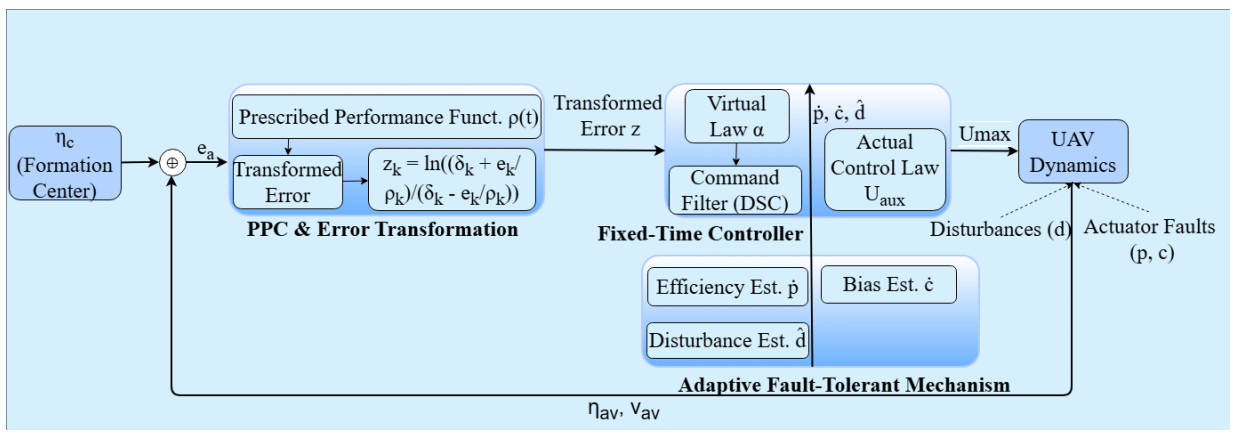
To achieve the desired tracking performance, the overall control architecture proposed in this paper is shown in Figure 2. It mainly consists of a trajectory tracking controller, a fault-tolerant mechanism, and a disturbance observer. PPC is an advanced control strategy designed to precisely regulate both transient and steady-state tracking performance. Its fundamental idea involves designing time-varying performance functions to establish strict boundaries for the error convergence process, thereby ensuring that overshoot, convergence rate, and steady-state precision satisfy predefined requirements.

Figure 2. Block diagram of the proposed fixed-time prescribed performance fault-tolerant control strategy for the UAV subsystem. The architecture integrates error transformation, command filtering, and adaptive compensation to handle safety constraints and actuator faults. UAV: Unmanned aerial vehicle; PPC: prescribed performance control; DSC: dynamic surface control.

In the proposed framework, the UAV tracks the geometric center of the USV formation as its target. Let the UAV position in the inertial frame be $$ \boldsymbol{\eta}_a = [x_a, y_a, z_a]^T $$, and the formation center position be $$ \boldsymbol{\eta}_c = [x_c, y_c, 0]^T $$. The formation tracking error, denoted as $$ \boldsymbol{e}_a $$, is defined as:

where $$ \Delta x_d $$ and $$ \Delta y_d $$ represent the desired horizontal offsets relative to the formation center, and $$ H_d $$ denotes the desired flight altitude.

Accordingly, the error dynamics are given by:

where $$ [v_{ax}, v_{ay}, v_{az}]^T $$ is the UAV velocity vector.

To achieve fixed-time convergence of tracking errors, a performance function $$ p_k(t) $$ is designed for each channel $$ k \in \{x, y, z\} $$. It defines the allowable evolution boundary of the tracking error:

where $$ p_{0k} $$ and $$ p_{\infty k} $$ represent the initial and the final (steady-state) values of the performance function, respectively, satisfying the condition $$ 0 < p_{\infty k} < p_{0k} $$. The function $$ \varphi(t) $$ is a specially designed polynomial decay function that ensures convergence within a fixed time $$ T_f $$:

Direct controller design based on the constrained error $$ \boldsymbol{e}_a $$ would result in complex nonlinear inequality constraints. Therefore, an evolution path and an error transformation function are introduced to convert the constrained problem into an unconstrained one.

The evolution path $$ Y_k(t) $$ is introduced as a “transitional trajectory” to guide the smooth convergence of the error. Its primary function is to eliminate initial error jumps (especially when the initial error is large) and to ensure smoothness of the control input.

The evolution path is designed as:

The introduction of $$ Y_k(t) $$ serves a critical role in handling initial errors. Unlike traditional PPC, where the initial error must be strictly within bounds, the evolution path ensures that $$ e(0) - Y(0) = 0 $$, eliminating the risk of “term explosion” in the control input at $$ t = 0 $$ due to large initial deviations. The parameter $$ n \geq 2 $$ is selected to ensure sufficient smoothness of the evolution path (i.e., its first- and second-order derivatives exist and are continuous over $$ t = 0 $$ and $$ t = T_c $$).

Here, $$ T_c $$ is the desired convergence time (matched with the performance function); $$ n \ge 2 $$ is a smoothness parameter; and $$ e_{0k} $$ is the initial error, ensuring that the path starts exactly from the initial error value.

Define the deviation between the actual error and the ideal evolution path as:

where $$ \varepsilon_k $$ satisfies the constraint $$ -\delta_k p_k(t) < \varepsilon_k < \delta_k p_k(t) $$, with $$ 0 < \delta_k \le 1 $$. To transform the constrained variable $$ \varepsilon_k $$ into an unconstrained one, the following nonlinear logarithmic transformation function is introduced:

The logarithmic function transforms the constrained error $$ \varepsilon_k $$ defined in the domain $$(-\delta_k p_k, \delta_k p_k)$$ into an unconstrained variable $$ z_k \in (-\infty, +\infty)$$. This transformation allows the subsequent controller design to proceed without explicitly handling inequality constraints.

Here, $$ z_k $$ represents the transformed unconstrained error. When $$ \varepsilon_k \in (-\delta_k p_k(t), \delta_k p_k(t)) $$, there exists a one-to-one mapping between $$ z_k $$ and $$ \varepsilon_k $$. Furthermore, as $$ \varepsilon_k \to \pm \delta_k p_k(t) $$, it follows that $$ z_k \to \pm \infty $$. This property inherently prevents the constraints from being violated.

Taking the time derivative of $$ z_k $$, we obtain:

where the intermediate term $$ r_k(t) $$ is given by:

This transformed dynamics $$ \dot{z}_k $$ will be used in the subsequent controller design to ensure system stability.

Based on the dynamics of the transformed error $$ \boldsymbol{z} $$, a hierarchical control strategy consisting of “virtual control” and “actual control” is adopted. To avoid the “explosion of terms” inherent in traditional backstepping methods when calculating high-order derivatives, a first-order command filter is introduced to achieve smooth and stable convergence.

First, the dynamics of the transformed error system can be expressed in vector form as:

where $$ \dot{\boldsymbol{\varepsilon}} = \dot{\boldsymbol{e}}_a - \dot{\boldsymbol{Y}} $$. The vector $$ \boldsymbol{\Pi} $$ and the Jacobian matrix $$ \boldsymbol{\Psi} $$ are defined as:

Virtual Control Law Design: The virtual control law $$ \boldsymbol{\alpha} $$ serves as the desired velocity reference. To ensure the stability of the position loop, $$ \boldsymbol{\alpha} $$ is designed as:

where $$ \boldsymbol{K}_1 $$ is a positive definite gain matrix, and $$ \dot{\boldsymbol{\eta}}_c = [\dot{x}_c, \dot{y}_c, 0]^T $$ represents the velocity of the formation center. Note that the virtual control law $$\alpha$$ is designed directly in the inertial frame to maintain consistency with the position error $$z$$, thus simplifying the backstepping control law without loss of generality.

Command Filter Design: Since the virtual control law $$ \boldsymbol{\alpha} $$ involves high-order derivatives of the error, directly using it for differentiation would cause severe fluctuations in the control input. Therefore, a first-order filter is introduced to smooth the virtual control signal:

where $$ \tau_f $$ is the filter time constant, and $$ \boldsymbol{\alpha}_f $$ denotes the smoothed desired velocity. Accordingly, the filter error $$ \boldsymbol{y} $$ and its dynamics are defined as follows:

Actual Control Law Design: Define the actual velocity tracking error as:

Based on the equation of UAV dynamics $$ m_a \dot{\boldsymbol{v}}_a = \boldsymbol{\rho} \boldsymbol{U}_a + \boldsymbol{c} + \boldsymbol{d}_a $$, and considering compensation for actuator faults and disturbances, the actual control law $$ \boldsymbol{U}_a $$ is designed as:

where $$ \boldsymbol{K}_2 $$ is a positive definite gain matrix for the velocity loop. $$ \hat{\boldsymbol{\rho}} $$, $$ \hat{\boldsymbol{c}} $$, and $$ \hat{\boldsymbol{d}}_a $$ are the adaptive estimates of the actuator efficiency matrix, bias fault, and lumped disturbances, respectively. The term $$ - \boldsymbol{\Psi}^T \boldsymbol{z} $$ is introduced to eliminate the coupling effects arising from the coordinate transformation during the stability analysis.

3.3. Adaptive update laws design

To estimate the unknown parameters $$ \boldsymbol{\rho} $$, $$ \boldsymbol{c} $$, and $$ \boldsymbol{d}_a $$ online, adaptive update laws are designed based on Lyapunov stability theory.

First, define the parameter estimation errors:

Consider the following Lyapunov candidate terms for parameter adaptation:

where $$ \boldsymbol{\Gamma}_\rho, \boldsymbol{\Gamma}_c, \boldsymbol{\Gamma}_d $$ are positive definite symmetric adaptive gain matrices.

Taking the time derivative of $$ V_\rho $$ yields $$ \dot{V}_\rho = \text{tr}(\tilde{\boldsymbol{\rho}}^T \boldsymbol{\Gamma}_\rho^{-1} \dot{\tilde{\boldsymbol{\rho}}}) = -\text{tr}(\tilde{\boldsymbol{\rho}}^T \boldsymbol{\Gamma}_\rho^{-1} \dot{\hat{\boldsymbol{\rho}}}) $$. To eliminate the cross-coupling terms appearing in the time derivative of the velocity error subsystem (specifically the term $$ \boldsymbol{s}^T \tilde{\boldsymbol{\rho}} \boldsymbol{U}_a $$), and to incorporate $$ \sigma $$-modification for preventing parameter drift, the adaptive update laws are designed as follows:

where $$ \boldsymbol{\Sigma}_\rho, \boldsymbol{\Sigma}_c, and \boldsymbol{\Sigma}_d $$ are positive design parameters for robust modification terms. These laws ensure that the estimates converge to a bounded region near their true values.

4.1. Fixed-time stability proof for USV formation

Construct the following composite Lyapunov candidate function:

where $$ \tilde{\boldsymbol{d}} = \boldsymbol{d} - \hat{\boldsymbol{d}} $$ represents the disturbance estimation error, $$ \boldsymbol{\Gamma}_p, \boldsymbol{\Gamma}_v > 0 $$ are positive definite diagonal gain matrices, and $$ \boldsymbol{M}_i $$ is the positive definite symmetric inertia matrix of the $$ i $$-th USV.

Taking the time derivative of the Lyapunov function $$ V $$ yields:

Step 1: Position Loop Dynamics. Substituting the kinematic equation and the virtual control definition, the derivative of the position error is derived as:

Recalling that $$ \boldsymbol{v}_i = \boldsymbol{e}_{vi} + \boldsymbol{v}_{id} $$, and expanding the virtual control law, we obtain:

where $$ \boldsymbol{u}_{pi} $$ contains the stabilizing feedback term and the compensation of the disturbance. Consequently, the first term in $$ \dot{V} $$ becomes:

Step 2: Velocity Loop Dynamics. Substituting the USV dynamics and the actual control law $$ \boldsymbol{\tau}_i $$ into the second term, it is crucial to note that, based on the backstepping design principle, the actual control law implicitly includes a compensation term $$ -\boldsymbol{R1}^T(\psi_i)\boldsymbol{e}_{pi} $$ to eliminate the coupling effect from the position loop. The closed-loop dynamics of the velocity error can be simplified as:

Thus, the second term in $$ \dot{V} $$ becomes:

From the above equations, it can be observed that the coupling term $$ \boldsymbol{e}_{pi}^T \boldsymbol{R1}(\psi_i)\boldsymbol{e}_{vi} $$ in the position loop exactly cancels with the term $$ -\boldsymbol{e}_{vi}^T \boldsymbol{R1}^T(\psi_i)\boldsymbol{e}_{pi} $$ in the velocity loop.

Step 3: Disturbance Estimation Error. Assuming that the external disturbance varies slowly relative to the observer dynamics, i.e., $$ \dot{\boldsymbol{d}} \approx 0 $$, we obtain $$ \dot{\tilde{\boldsymbol{d}}} = -\dot{\hat{\boldsymbol{d}}} $$. Substituting the observer update laws:

These observer dynamics are designed to stabilize the estimation error subsystem within a fixed time.

Substituting all terms back into $$ \dot{V} $$, and using the fixed-time stability properties of $$ \boldsymbol{u}_{pi} $$ and $$ \boldsymbol{u}_{vi} $$ (which contain terms such as $$ -k_1 \text{sig}^{\alpha_1}(\boldsymbol{e}) - k_2 \text{sig}^{\alpha_2}(\boldsymbol{e}) $$), it can be proven that the time derivative of the Lyapunov function satisfies the following fixed-time stability condition:

Remark 3: Since the residual term $$ C $$ satisfies $$ C > 0 $$, the system achieves practical fixed-time stability (P-FTS) rather than exact asymptotic convergence to zero. The tracking error converges to a neighborhood of the origin $$ \Omega_e $$ within a bounded settling time $$ T_{max} $$. The upper bound of the settling time is estimated as:

where $$ 0 < \theta < 1 $$ is a scalar parameter. The convergence region is bounded by the set where the stabilizing terms dominate the residual term $$ C $$.

Here, $$ \mu_1, \mu_2 > 0 $$, and $$ C $$ is a small residual constant. This inequality guarantees that the tracking errors $$ \boldsymbol{e}_{pi} $$ and $$ \boldsymbol{e}_{vi} $$ converge to a small neighborhood of the origin within a fixed time $$ T_{\max} $$, independent of the initial states.

4.2. Stability proof for the UAV subsystem

Construct the following composite Lyapunov candidate function:

where the components are defined as:

5.1. Simulation setup

The simulations are performed using MATLAB with a fixed time step of $$ dt = 0.005 $$ s over a duration of $$ t = 30 $$ s. The heterogeneous system comprises $$ N = 4 $$ USVs and a single UAV.

5.2. Comparative analysis of UAV trajectory

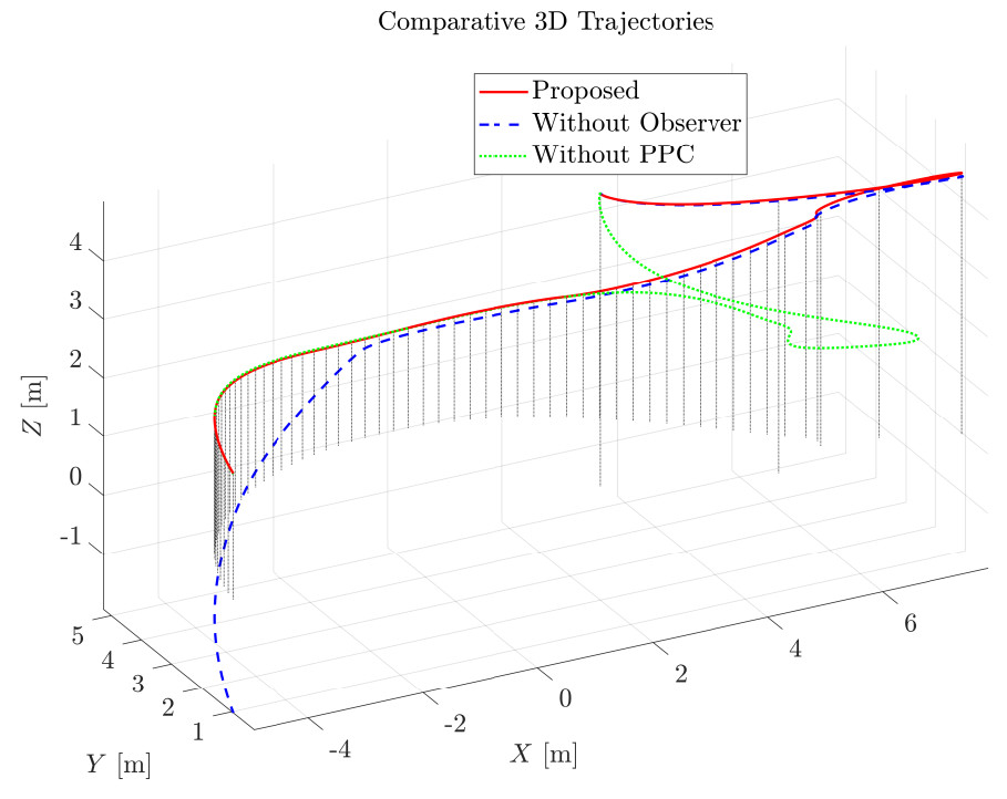
Figure 3 presents a comparison of the 3D trajectories of the heterogeneous system. The Proposed method (red solid line) follows the spiral ascending track easily and sustains the formation structure perfectly. In contrast, the Without PPC case (green dotted line) exhibits pronounced oscillations in the initial stage due to the absence of transient constraints. Most importantly, in the Without Observer case (blue dashed line), the UAV suffers from a severe altitude drop (Z-axis). This is because the 10% thrust loss ($$ \rho = 0.9 $$) remains uncompensated, preventing the system from generating sufficient lift to counteract gravity, confirming the necessity of the "fault-tolerant" nature of our design. It is crucial to clarify that a 10% efficiency loss is not an exaggerated fault setting. Because rotary-wing UAVs rely entirely on actuator-generated thrust to counteract gravity, their steady-state thrust margin is strictly limited. An uncompensated 10% loss in total lifting capability directly disrupts the delicate balance required for hovering and altitude tracking, inevitably leading to the pronounced altitude deviation observed. This physical constraint underscores the critical need for the proposed adaptive observer.

Figure 3. Comparative 3D trajectories. The Proposed method (red) tracks the reference smoothly, while the Without Observer case (blue) suffers from altitude deviation. PPC: Prescribed performance control.

5.3. Comparative error analysis of UAV

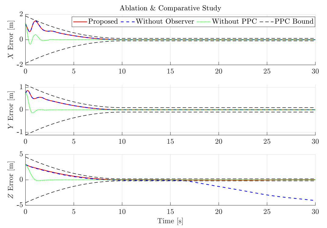
Figure 4 provides a more detailed understanding of control quality. Transient Smoothness: While the Without PPC case (green) stays within the boundaries in this setup, it exhibits pronounced jitter and non-smooth "sharp turns" in the X and Y channels during the first 2 s. In contrast, the Proposed method (red) follows the Ideal Evolution Path (grey dots) with superior smoothness. Boundary Enforcement: The PPC boundaries (black dashed lines) strictly envelope the red trajectory. Critical Failure Analysis: In the Z-error subplot, the Without Observer case (blue) diverges significantly after $$ t=15 $$ s, eventually violating the PPC boundary. This proves that without the adaptive observer, even the PPC mechanism cannot prevent system failure under persistent actuator faults.

Figure 4. Comparative evolution of UAV tracking errors. Black dashed lines indicate PPC boundaries. UAV: Unmanned aerial vehicle; PPC: prescribed performance control.

5.4. UAV parameter identification

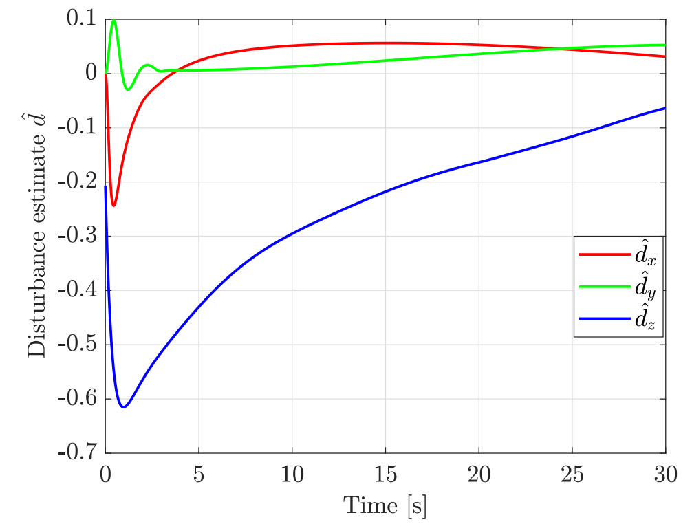
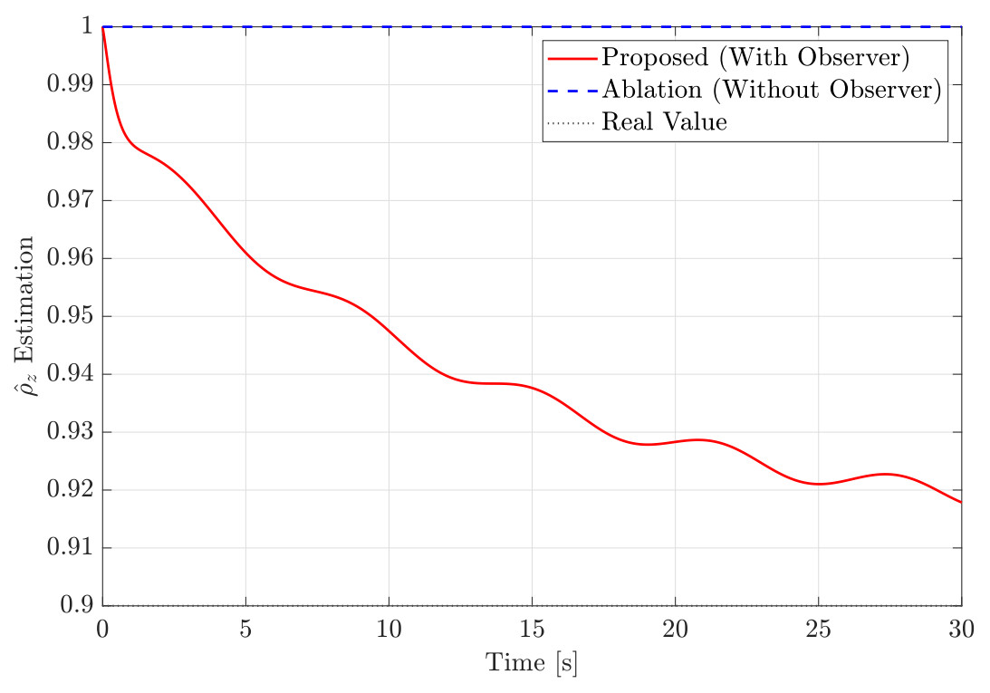
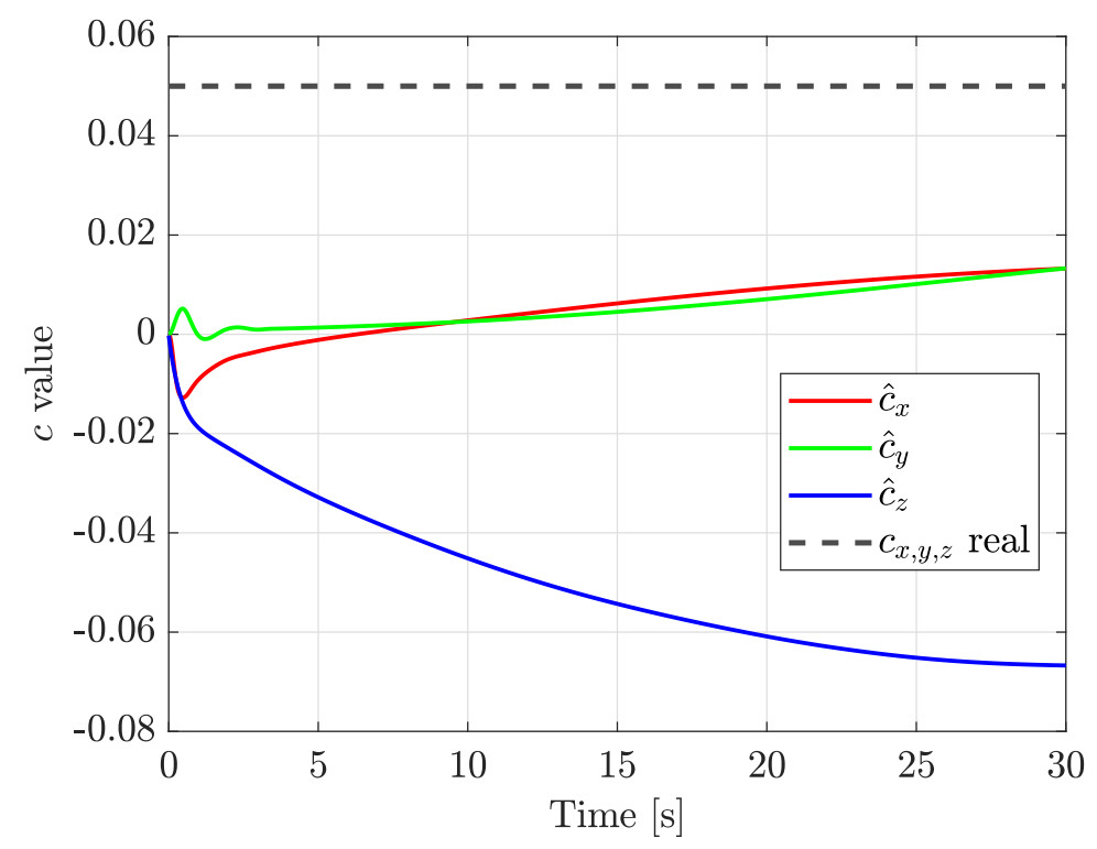
Figure 5 illustrates the performance of the observer. For the Proposed case, the efficiency estimate $$ \hat{\rho}_z $$ successfully converges from 1.0 to approximately 0.915, closely tracking the true fault value of 0.9. The small residual error is due to the robust $$ \sigma $$-modification. In contrast, the Ablation case (blue) remains at 1.0, indicating that the actuator degradation cannot be detected. As shown in Figure 6, the bias estimate $$ \hat{c} $$ does not exhibit divergence or saturation and stabilizes around -0.06. Although there is a steady-state deviation from the set true value of 0.05, this is acceptable in adaptive control theory. Due to the parameter redundancy among $$ \rho $$, $$ c $$, and $$ d $$, the controller compensates for the overall error through coordinated adjustments of these parameters (e.g., a slightly higher $$ \hat{\rho} $$ accompanied by a lower $$ \hat{c} $$). The estimated values remain bounded, ensuring the stability of the control system. Figure 7 is a critical graph to validate the accuracy of the physical model. The estimated values converge to approximately -0.1 (close to 0) rather than the gravitational acceleration component (-9.8). This result provides strong evidence that the gravity feedforward compensation in the controller is correct. Consequently, the observer is only responsible for estimating the minute air resistance and residual modeling errors, reflecting the high fidelity of the model.

Figure 5. Adaptive estimation of UAV actuator efficiency $$ \rho_z $$. UAV: Unmanned aerial vehicle.

Figure 6. Estimation of UAV actuator bias faults ($$ \hat{c} $$). UAV: Unmanned aerial vehicle.

Figure 7. Estimation of lumped disturbances ($$ \hat{d} $$) affecting the UAV. UAV: Unmanned aerial vehicle.

Remark 5 (Comprehensive analysis on parameter estimation and control objectives):

As shown in Figure 6, the estimated bias $$ c $$ stabilizes at $$-0.06$$, which differs from the true injected value of $$0.05$$. It is crucial to clarify that this deviation does not invalidate the physical meaning of the controller, nor does it affect the system stability. This phenomenon is explained from three main aspects:

First, regarding parameter identifiability, the bias fault $$ c $$ and the lumped disturbance $$ d_a $$ are dynamically coupled, as they affect the UAV system through the exact same control input channel. In standard adaptive control theory, strict convergence of multiple coupled parameters to their true physical values requires the system states to satisfy the persistently exciting (PE) condition. However, achieving PE typically necessitates injecting rich, high-frequency signals into the trajectory, which would cause severe and unacceptable chattering during actual UAV flight. Without the PE condition, individual parameters are not strictly identifiable.

Second, regarding the reasonableness of the framework, such non-convergence to true values is a standard and acceptable characteristic of robust adaptive control. The robust $$ \sigma $$-modification applied in the adaptive update laws [Equations (49) and (50)] guarantees that estimates will not drift to infinity but remain strictly bounded. The adaptive mechanism and the disturbance observer collaboratively compensate for the algebraic sum of uncertainties. As shown in Figure 7, $$ d_a $$ converges to approximately $$-0.1$$. The overall dynamic compensation provided by the controller is $$-0.06 + (-0.1) = -0.16$$, which effectively neutralizes the true combined uncertainty acting on the system channel.

Finally, regarding the control objective, the primary goal of the proposed fixed-time PPC is trajectory tracking and ensuring that errors remain strictly within safety boundaries, rather than performing precise system parameter identification. The Lyapunov-based stability analysis in Section 4 theoretically proves that tracking stability and error constraints are guaranteed as long as the overall uncertainty is compensated and the estimation errors remain bounded, completely independent of whether individual parameters converge to their exact physical true values.

5.5. Performance of USV formation (fixed-time stability)

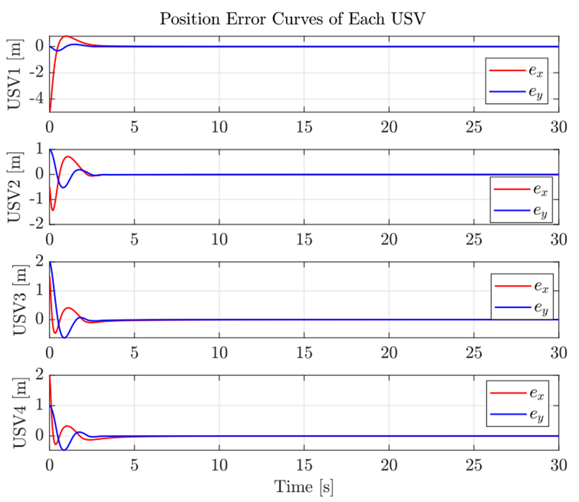
Figure 8 illustrates the position tracking error curves of the four USVs during the formation process. The initial position errors of the followers (about 5 m) quickly converge to zero within an extremely short time interval ($$ t < 3 $$ s). In the steady state, the position tracking error is on the order of $$ 10^{-3} $$ and the convergence process is smooth, without any oscillations. These results show that the proposed fixed-time control law achieves a high convergence speed, enabling the USV formation to complete reconfiguration and reach a stable formation-keeping state in less than 3 s.

Figure 8. Convergence curves of position tracking errors for each autonomous vehicle. USV: Unmanned surface vehicle.

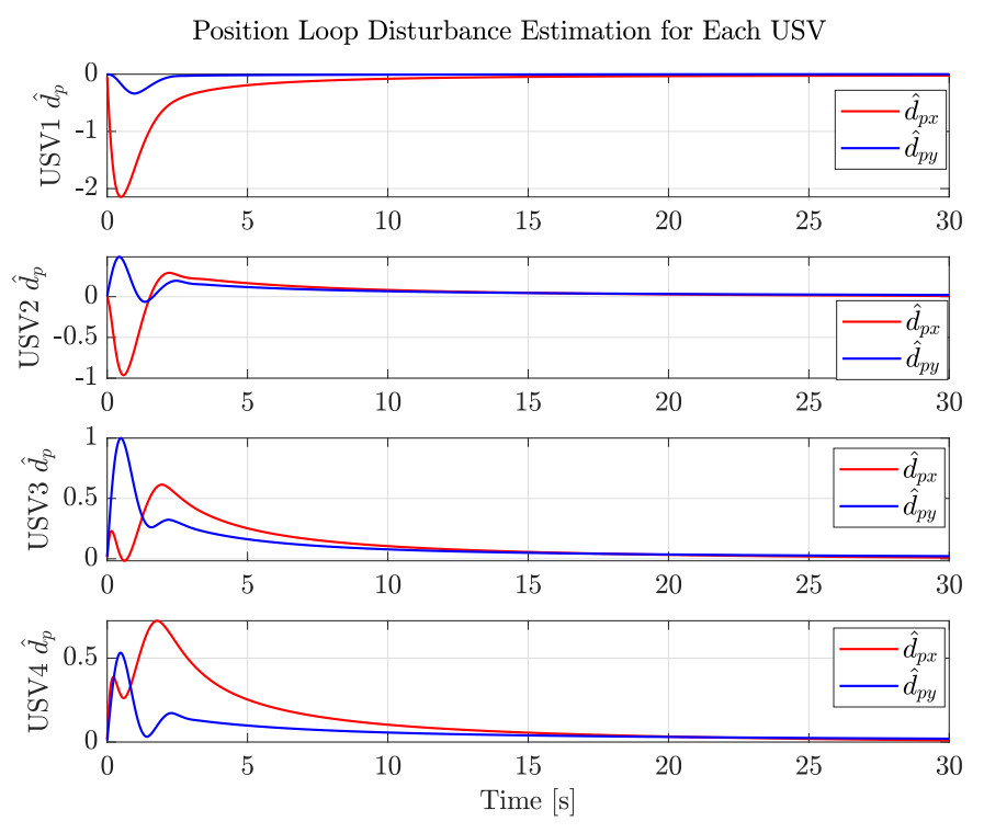
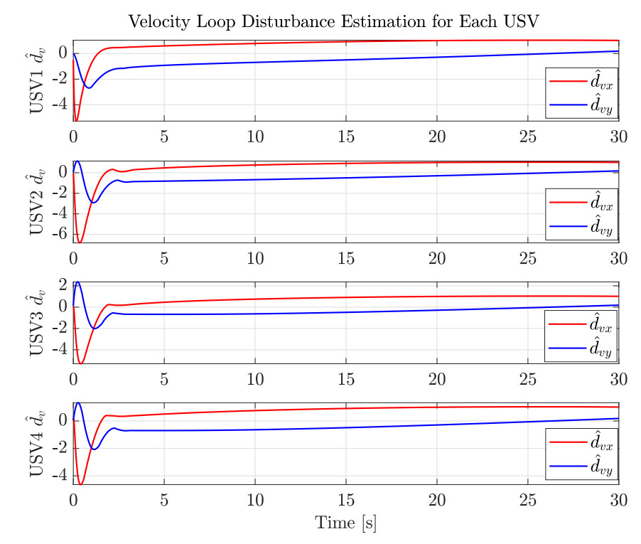
Figures 9 and 10 display the estimation results of the disturbance observers for the USV position loop and velocity loop, respectively. For the position loop disturbance estimates [Figure 9], the observed values converge to the steady state within 5 s, effectively capturing environmental disturbances such as currents.

Figure 9. USV position loop disturbance estimation results. USV: Unmanned surface vehicle.

Figure 10. USV velocity loop disturbance estimation results. USV: Unmanned surface vehicle.

For the velocity loop disturbances [Figure 10], different USVs (e.g., USV1 vs. USV2) experience different linear velocities due to their positions in the inner and outer lanes of the formation during turning maneuvers, leading to varying hydrodynamic drag forces. The estimated disturbance curves accurately reflect this physical phenomenon, converging to distinct constant values (ranging between -1 and +1). This proves that the observer can precisely capture model uncertainties under different dynamic states.

It is worth noting that, to clearly verify the baseline convergence and steady-state tracking performance of the proposed disturbance observers, the environmental disturbances in this simulation case are primarily modeled as steady-state components (e.g., constant ocean currents and mean wind forces). As shown in the results, the proposed observers rapidly and accurately converge to these constant principal values, demonstrating excellent steady-state estimation performance. Validating the system's robustness against higher-frequency, violently fluctuating wave dynamics remains an important aspect of future real-world experiments.

Authors’ contributions

Made substantial contributions to the conception and design of the study and performed data analysis and interpretation: Liang, Z.; Zhou, W.; Wang, Y.

Performed data acquisition, as well as providing administrative, technical, and material support: Wang, Y.; Yang, Y.

Availability of data and materials

All simulation parameters and mathematical models used to support the findings of this study are included within the article.

AI and AI-assisted tools statement

During the preparation of this work, the authors used AI-assisted tools, specifically ChatGPT (version GPT-4, OpenAI), for language translation, text polishing to improve readability, and visual enhancement of block diagrams (e.g., layout optimization and formatting). The conceptual content, mathematical modeling, data generation, and all scientific results are entirely the original work of the authors. After using these tools, the authors thoroughly reviewed and edited both the manuscript and figures, and take full responsibility for the final content of the publication. No AI technologies were used in the study design, mathematical modeling, or generation of data and results.

Financial support and sponsorship

This work was supported by the National Natural Science Foundation of China (Grant Nos. 62203293 and 52407123) and the Social and People's Livelihood Science and Technology Project (Grant No. MSZ2025119).

Conflicts of interest

All authors declared that there are no conflicts of interest.

Ethical approval and consent to participate

Not applicable.

Consent for publication

Not applicable.

Copyright

© The Author(s) 2026.

REFERENCES

1. Ren, H.; Liu, Q.; Zhou, Q.; Lu, R. A review of distributed cooperative control research on unmanned autonomous systems (in Chinese). J. Guangdong. Univ. Technol. 2024, 41, 1-13.
2. Xiong, Y.; Fu, M.; Li, B.; Yao, T.; Zhang, R. Multi-robot formation control based on leader-follower method (in Chinese). Mech. Electr. Eng. Technol. 2024, 53, 136-41. https://kns.cnki.net/kcms2/article/abstract?v=zE0--Q1IihSpR58jxWP-rI_Xt7XR2FFHu_0U64TvMTFY-xHgpaKYdipE-eFxbuLPGSU-Ef381kUv8Eb-Sohrv5y4Fntr8xVUXS49IIXdEAUhJXWsmxq3FSgyF7K9TbzRDnTjFc-J7R_WyHY983wtH9eT2GIu6MA-yHQIM3RsrXRywMCnN1Pw_w==&uniplatform=NZKPT&language=CHS. (accessed 2026-05-12).
3. Piracha, A. Z.; Rinner, B. Virtual leader-based safe formation-switching control for dense environments. In ICASSP 2025 - 2025 IEEE International Conference on Acoustics, Speech and Signal Processing (ICASSP), Hyderabad, India. Apr 06-11, 2025. IEEE; 2025. p. 1-5.
4. Luo, D.; Wang, Y.; Lewis, F. L.; Song, Y. Unified output feedback based prescribed performance consensus tracking control of heterogeneous multi-agent systems. IEEE/CAA. J. Autom. Sin. 2025, 12, 1636-47.
5. Wu, Y.; Low, K. H.; Lv, C. Cooperative path planning for heterogeneous unmanned vehicles in a search-and-track mission aiming at an underwater target. IEEE. Trans. Veh. Technol. 2020, 69, 6782-7.
6. Huang, T.; Chen, Z.; Gao, W.; Xue, Z.; Liu, Y. A USV-UAV cooperative trajectory planning algorithm with hull dynamic constraints. Sensors 2023, 23, 1845.
7. Zhang, J.; Liu, X.; Wang, X.; Wang, Y.; Wang, Y. Adaptive prescribed performance tracking control for underactuated unmanned surface ships with input quantization. Intell. Robot. 2024, 4, 146-63.
8. Li, J.; Zhang, G.; Zhang, X.; Zhang, W. Integrating dynamic event-triggered and sensor-tolerant control: application to USV-UAVs cooperative formation system for maritime parallel search. IEEE. Trans. Intell. Transp. Syst. 2024, 25, 3986-98.
9. Li, J.; Zhang, G.; Wang, L.; Zhang, X. Modeling and cooperative path following control of USVs-UAVs via the event-triggered communication. In 2024 36th Chinese Control and Decision Conference (CCDC), Xi'an, China. May 25-27, 2024. IEEE; 2024. pp. 1568-72.
10. Li, X.; Cai, G.; Wu, T.; Yang, Q. A formation transformation control method for UAV swarm based on stress matrix (in Chinese). Control. Decis. 2024, 39, 2195-204.
11. Roggi, G.; Gozzini, G.; Invernizzi, D.; Lovera, M. Vision-based air-to-air autonomous landing of underactuated VTOL UAVs. IEEE/ASME. Trans. Mechatronics. 2024, 29, 2338-49.
12. He, X.; Li, Y.; Yu, Y. Prescribed-time formation control of quadrotor UAVs based on leader-follower approach (in Chinese). Control. Eng. China. 2025, 32, 1813-21.
13. Li, X.; Wen, G.; Sun, C. Leader-following consensus of open multi-unmanned aerial vehicles systems under directed topology. In 2024 SICE Festival with Annual Conference (SICE FES), Kochi City, Japan. Aug 27-30, 2024. IEEE; 2024. pp. 752-7. https://ieeexplore.ieee.org/document/10805206. (accessed 2026-05-12).
14. Sun, Y.; Peng, S. Consensus of discrete-time leader-following linear multi-agent systems under Lyapunov-function-based event-triggered mechanism. IEEE. Trans. Circuits. Syst. Ⅱ. Exp. Briefs. 2023, 70, 4409-13.
15. Song, S.; Liu, Z.; Yuan, S.; Wang, Z. Cascaded extended state observers-based fixed-time line-of-sight path following control for unmanned surface vehicles with disturbances and saturation. IEEE. Trans. Veh. Technol. 2024, 73, 7733-47.
16. Gao, H.; Xia, Y.; Liu, K.; Zhang, J.; Cui, B. Resilient neuroadaptive distributed fixed-time attitude coordination control for multiple spacecraft. IEEE. Trans. Cybern. 2024, 54, 4973-85.
17. Wang, T.; Xu, Y.; Liu, Y.; Wang, D. Fast fixed-time-synchronized sliding mode formation control for uncertain autonomous surface vehicles. In 2025 37th Chinese Control and Decision Conference (CCDC), Xiamen, China. May 16-19, 2025. IEEE; 2025. pp. 1664-9.
18. Zhang, J.; Yu, S.; Yan, Y.; Wu, D. Fixed-time output feedback sliding mode tracking control of marine surface vehicles under actuator faults with disturbance cancellation. Appl. Ocean. Res. 2020, 104, 102378.
19. Shang, Y.; Ye, Y. Fixed-time group tracking control with unknown inherent nonlinear dynamics. IEEE. Access. 2017, 5, 12833-42.
20. Shang, Y. Fixed-time group consensus for multi-agent systems with non-linear dynamics and uncertainties. IET. Control. Theory. Appl. 2018, 12, 395-404.
21. Sun, G.; Liang, B. Fixed-time observer based adaptive prescribed performance control for full state feedback system with disturbance. In 2024 IEEE 13th Data Driven Control and Learning Systems Conference (DDCLS), Kaifeng, China. May 17-19, 2024. IEEE; 2024. pp. 848-53.
22. Peng, Y.; Yan, H.; Rao, K.; Yang, P.; Lv, Y. Distributed model predictive control for unmanned aerial vehicles and vehicle platoon systems: a review. Intell. Robot. 2024, 4, 293-317.
23. Ding, J.; Zhang, H. T.; Hu, B. B.; Jiang, W.; Liu, X. Mutual-rendezvous control and feature-compatible landing optimization for heterogeneous UAV–USV fleets. IEEE. Trans. Ind. Inform. 2026, 22, 348-59.
24. Luo, Y.; Tang, F.; Wei, Q. Event-based human-in-the-loop formation-containment control for heterogeneous UAV-USV systems with dual predefined-time prescribed performance. IEEE. Trans. Veh. Technol. 2026, 75, 1990-2000.
25. Li, S.; Jia, Y.; Xiang, Z.; Zhang, J. Distributed event-triggered positive consensus protocol design for leader-following multi-agent systems. In 2025 IEEE 14th Data Driven Control and Learning Systems (DDCLS), Wuxi, China. May 09-11, 2025. IEEE; 2025. pp. 398-403.
26. Su, W.; Mu, C.; Zhu, S.; Niu, B.; Sun, C. Event-triggered leader-follower bipartite consensus control for nonlinear multi-agent systems under DoS attacks. Sci. China. Inf. Sci. 2025, 68, 132206.
27. Wu, Y.; Liang, H.; Xuan, S.; Zhang, X. Extended state observer based finite-time fault-tolerant formation control for multi-UAVs. J. Franklin. Inst. 2024, 361, 107158.
28. Zhang, H.; Ding, Y.; Yue, X. Distributed formation control of aircraft with fixed-time and prescribed performance based on leader-follower approach (in Chinese). Aeronaut. Sci. Technol. 2025, 36, 1-9.
29. Zheng, Z.; Wang, Y.; Li, C. Observer-based fixed-time leader-following consensus control for MASs subject to DoS attack. In 2023 7th International Symposium on Computer Science and Intelligent Control (ISCSIC), Nanjing, China. Oct 27-29, 2023. IEEE; 2023. pp. 236-40.
30. Trejo, J. A. V.; Ponsart, J. C.; Adam-Medina, M.; Valencia-Palomo, G.; Theilliol, D. Distributed observer-based leader-following consensus control for LPV multi-agent systems: application to multiple VTOL-UAVs formation control. In 2023 International Conference on Unmanned Aircraft Systems (ICUAS), Warsaw, Poland. Jun 06-09, 2023. IEEE; 2023. p. 1-8.
31. Yang, Y.; Shen, B.; Ge, X.; Li, S.; Han, Q. L. Dynamic event-triggered cluster consensus of multi-agent systems via PSO-GA co-design. IEEE. Trans. Autom. Sci. Eng. 2025, 22, 11505-18.
32. Yang, T.; Lu, Z.; Cui, G.; Ding, S. Funnel-based predefined-time formation control for heterogeneous vehicle platoon with asymptotic tracking. IEEE. Trans. Veh. Technol. 2025, 74, 7178-87.
33. Ballotta, L.; Talak, R. Safe distributed control of multi-robot systems with communication delays. IEEE. Trans. Veh. Technol. 2025, 74, 10137-50.
34. Wang, H.; Wang, H.; Guo, X. Distributed adaptive fault-tolerant formation control for heterogeneous USV-AUV swarms based on dynamic event triggering. J. Mar. Sci. Eng. 2025, 13, 2116.
35. Ma, Y.; Jiang, B.; Wang, J.; Gong, J. Adaptive fault-tolerant formation control for heterogeneous UAVs-UGVs systems with multiple actuator faults. IEEE. Trans. Aerosp. Electron. Syst. 2023, 59, 6705-16.
36. Yang, Z.; Li, M.; Yu, Z.; Cheng, Y.; Xu, G.; Zhang, Y. Fault detection and fault-tolerant cooperative control of multi-UAVs under actuator faults, sensor faults, and wind disturbances. Drones 2023, 7, 503.
37. Yang, Y.; Zhang, B.; Hu, M. Heterogeneous formation control of UAV-USV under actuator faults (in Chinese). Flight. Control. Detect. 2024, 7, 14-20.
38. Charitidou, M.; Dimarogonas, D. V. Virtual leader and distance based formation control with funnel constraints. IEEE. Trans. Control. Netw. Syst. 2025, 12, 1342-53.
39. Imran, I. H.; Kurtulus, D. F.; Memon, A. M.; Goli, S.; Kouser, T.; Alhems, L. M. Distributed robust formation control of heterogeneous multi-UAVs with disturbance rejection. IEEE. Access. 2024, 12, 55326-41.
40. Zhang, J.; Yu, S.; Yan, Y.; Zhao, Y. Fixed-time trajectory tracking control for marine surface vessels based on fixed-time disturbance observer. In 2020 5th International Conference on Automation, Control and Robotics Engineering (CACRE), Dalian, China. Sep 19-20. 2020. IEEE; 2020. pp. 308-12.
Cite This Article
Research Article