



Integrated PredRNN++ and phase-field for microstructure prediction and simulation acceleration
 0
0 Abstract
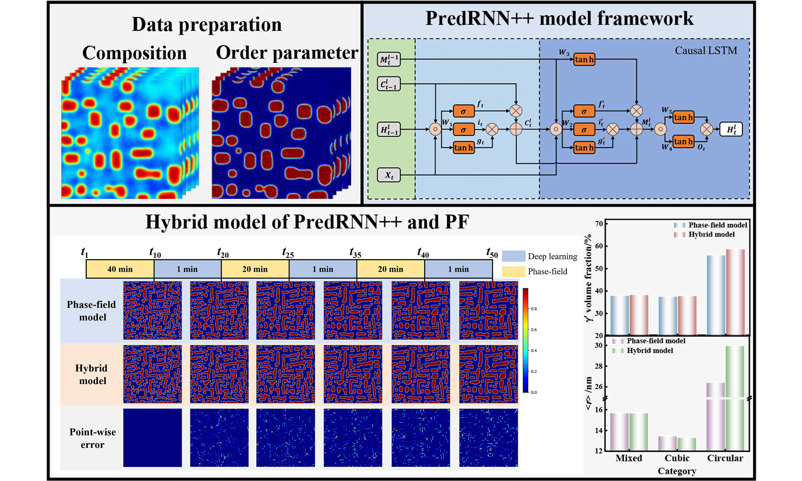
Deep learning methods are integrated with phase-field (PF) simulations to predict microstructural evolution and accelerate PF simulations, thereby overcoming the high computational cost associated with multi-parameter, multi-component parameter optimization. The predictive recurrent neural network++ (PredRNN++) model is developed to predict the precipitation morphologies with circular, cubic and mixed-shape accompanying the growth and coarsening process in superalloys. Compared with convolutional long short-term memory, predictive recurrent neural network, and convolutional neural network models, the PredRNN++ model shows superior prediction performance in precipitate microstructural evolution. Moreover, the hybrid model of PredRNN++ and PF is developed to accelerate the prediction of precipitate evolution, the computational efficiency of the hybrid model exceeds 2.9 times that of the single PF model. In the hybrid model, the calculation speed of PredRNN++ is 40 times that of the PF, and the mean square error remains within 0.004. In particular, it enables the analysis of precipitation kinetics in mixed-shaped precipitates. The advantages of the PredRNN++ model are discovered in predicting the precipitate microstructures, accompanied by Ostwald ripening and coalescence coarsening mechanisms. This study advances the applicability of deep learning to complex microstructural evolution and the feasibility of accelerating PF simulations.
Keywords
INTRODUCTION
The material microstructure is crucially linked with composition and macroscopic properties, making it a key factor in materials research. Phase-field (PF) methods[1,2], a powerful mesoscale simulation technique, are employed to predict microstructural evolution and deepen understanding of morphological dynamics, such as solidification[3,4], crystal growth[5-7], and solid-state phase transformation[8,9]. Continuous field variables represent the morphologies obtained from PF simulations, the Cahn-Hilliard[10] or Ginzburg-Landau[11] equations are utilized to control the field variables, incorporating with the finite-difference[12], the Runge-Kutta[13], the semi-implicit Fourier-spectral[14], and finite element methods[15,16] to solve the partial differential equations (PDEs). This process requires accurate temporal and spatial discretization of the field variables to ensure solution convergence and high-fidelity morphology[14]. Additionally, the PF model requires numerous input parameters. Therefore, accurately capturing PF microstructural evolution is computationally expensive and challenging, especially in multi-component, multi-field-coupling studies.
To address this problem, adaptive mesh refinement algorithms[17,18], parallel computing, and multi-scale model coupling methods[19] have been employed to accelerate PF calculations. For instance, the proper orthogonal decomposition (POD) combined with the Galerkin projection is used as a dimensionality reduction technique to mitigate the computational cost of high-fidelity numerical simulation[20,21]. Recently, machine learning has been widely applied in materials science[22-25], including predicting material properties and crystal structures[26-30], designing new materials[31-34], classification[35-40], and identification[41,42] of material microstructure. Consequently, some scholars have proposed numerical methods for solving partial differential equations, such as using machine learning models to replace PF simulations and inferring the accurate evolution process from input morphological data.
Traditional machine learning models are not suitable for large-scale data computations. Common replacement models include multilayer perceptron (MLP), convolutional neural network (CNN)[43,44], recurrent neural network (RNN)[45-47] and long short-term memory (LSTM)[43,48,49]. These methods have achieved significant performance on solving partial differential equations. Gesch et al. used autoencoder-based recurrent neural networks to predict the microstructural evolution of Ostwald ripening[49]. Oommen et al. employed the DeepONet model to replace the high-fidelity PF numerical solver in two-phase microstructural evolution[50]. Teichert et al. used machine learning algorithms to represent high-dimensional free energy surfaces to identify precipitate morphologies in alloy systems[51]. CNN can effectively capture spatial features but lacks explicit modeling capabilities for time series. RNN and LSTM often suffer from gradient vanishing/exploding problems when processing long sequences, making it difficult to capture such long-term dynamic dependencies. These models are often used for simple processes, such as dendrite growth, spinodal decomposition and Ostwald ripening[52]. The machine learning models are used to predict simple morphologies and single-variable fields where microstructural evolution is straightforward. These methods have not yet been applied in more complex kinetics processes or multi-field systems. Therefore, this study was motivated by the complex aging processes of superalloys, which involve more than 50 precipitated phase particles and multiple order parameters and composition fields.
In this study, we propose a new deep learning model, PredRNN++ model, for predicting the precipitation microstructural evolution in superalloys and compare its performance with alternative models, such as CNN, RNN, and LSTM, demonstrating the advantage of PredRNN++ on solving partial differential equations of microstructural evolution. A hybrid computational model integrating PF and PredRNN++ is built, thereby significantly accelerating computation while preserving microstructural accuracy. Additionally, by employing different precipitate morphologies, the model’s adaptability to the evolution of precipitation microstructure in superalloys is examined.
MODELS AND METHODS
PF model
The Cahn-Hilliard and Ginzburg-Landau equations are used in the PF simulation for precipitates evolution in superalloys, these control the evolutions of composition field ci (r, t) and order parameter field ηp (r, t)[8].
where ξc (r, t) and ξη (r, t) are noise items in composition and order parameters, Vm is the molar volume of the alloy, F is the total energy, Mi are the chemical mobilities of different elements, and L is the interface mobility. These noise items are introduced to induce the initial nucleation and satisfy the fluctuation-dissipation theorem. The noise term is removed after the nucleation, so it has no impact on deep learning models for the long time aged phase morphology. Detailed PF model is given in the Supplementary Materials, where the parameters for PF simulation are shown in Supplementary Table 1.
PredRNN++ neural network model
PredRNN++ is an advanced neural network model designed explicitly for video prediction and future frames[53]. PredRNN++ consists of a cascading operation of spatiotemporal memory units (Causal LSTM) and the gradient highway unit (GHU) framework. The Causal LSTM structure features cascaded dual memory units that enable information transfer in both horizontal and vertical directions, addressing the challenge of learning from sequences in which spatial and temporal patterns are tightly intertwined. The GHU captures long-term memory dependencies by merging GHU modules, which can solve the potential problem of gradient vanishing. Compared to convolutional long short-term memory (ConvLSTM) and predictive recurrent neural network (PredRNN)[54,55], it has a more complex model architecture to achieve better predictive performance.
Figure 1A shows the Causal LSTM framework. A Causal LSTM unit includes dual memories: temporal memory
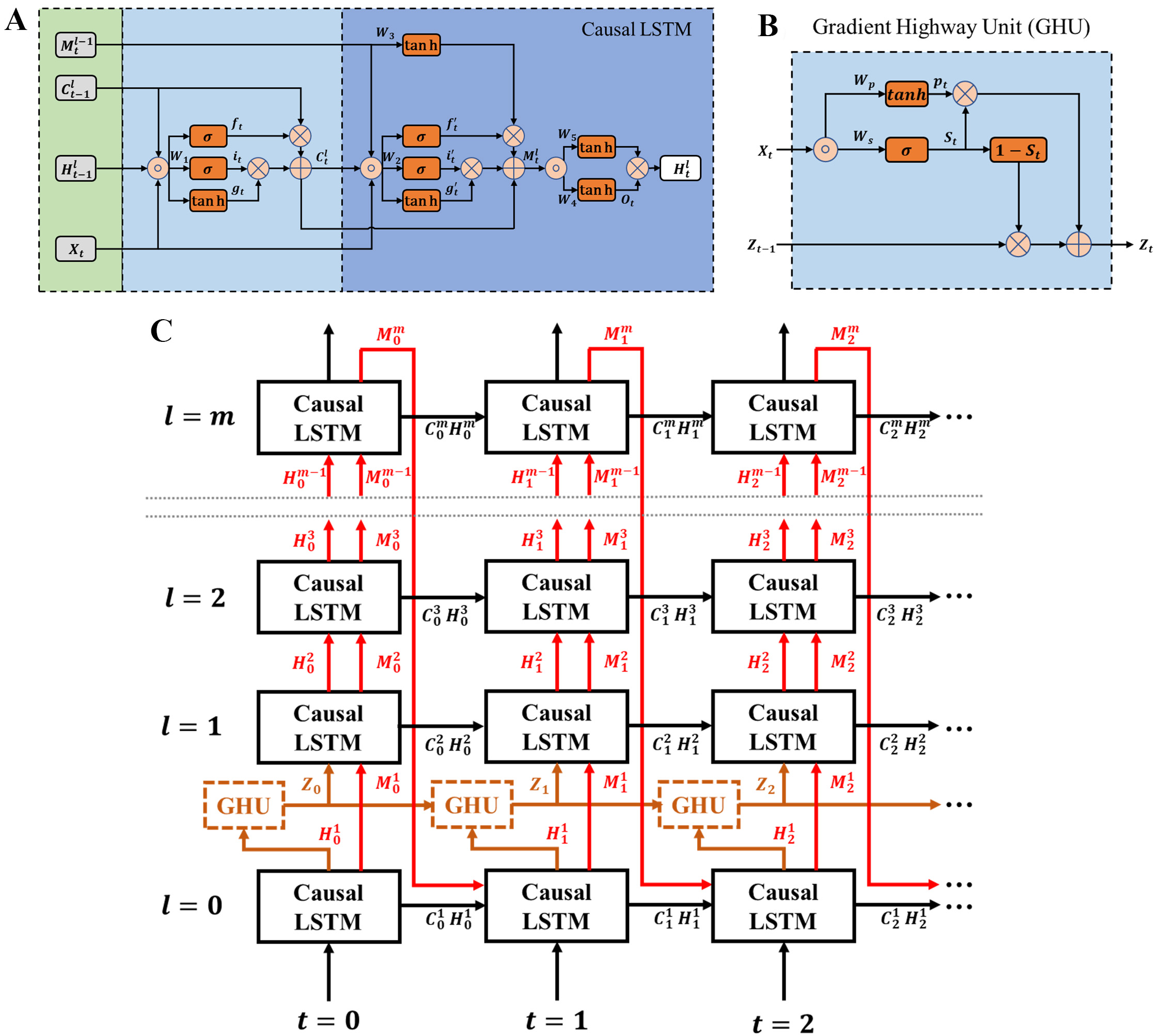
Figure 1. Schematic representation of the PredRNN++ model, (A) Causal LSTM framework, (B) GHU framework, (C) PredRNN++ framework integrating Causal LSTM and GHU. PredRNN++: Predictive recurrent neural network++; LSTM: long short-term memory; GHU: gradient highway unit.
where l is the current model layers, t is the specific time step in the sequence, Xt is the current input,
Figure 1B shows the GHU framework. This framework presents a novel spatiotemporal recurrent structure that effectively propagates gradients in deep feedforward networks. The GHU shows a rapid alternative route from the first to the last time step (the brown line in Figure 1C) to preserve the early information lost by
where Pt is the transformed inputs, St is the control gate,
Figure 1C shows the PredRNN++ framework that integrates Causal LSTM and GHU. It stacks m Causal LSTMs and inserts a GHU between the first and second layers of the Causal LSTMs. In this architecture, the gradient highway collaborates with Causal LSTM to utilize the rapidly updated hidden state Zt to capture both long- and short-term video dependencies. The equations are expressed as,
Data processing
To generate a diverse and extensive dataset for training deep learning models, isometric sampling was used. The interval between each time step is 10,000 iterations for the PF calculation. With initial composition of aluminum cAl ranging from 0.154 to 0.159, intervals of 0.001, and the interfacial free energy coefficients from 0.05 to 0.10, intervals of 0.01. These parameters are used in the aging simulation of superalloys. The testing set included cAl = 0.159 and all interfacial energy coefficients. The specific data details are shown in Supplementary Table 2. Due to the initial fluctuations, we select microstructural evolution from the stable state for the deep learning. The initial fluctuations only be added in the nucleation stage. Our PF-ML (machine learning) regimes are performed in the stable stage of phase evolution, in which the fluctuations are already removed. The initial fluctuation makes the high value of order parameters, while they go into stable development after that. Therefore, data from the first five time steps are excluded from the deep learning model. Then, the Min-Max normalization method is adopted. The order parameter field was directly normalized, while the composition field was first averaged to avoid inconsistent compositions before normalization. Finally, to further expand the dataset size and reduce computational cost, the 256×256 grids were divided into four cells with 128×128 grid. The calculation is performed by,
Where
The relevant tests, as shown in Supplementary Figure 1 [Supplementary Materials], and found that the volume fraction and particle distribution of the microstructures with or without partition were very similar.
To evaluate the performance of the model from multiple perspectives, the mean absolute error (MAE), mean square error (MSE), relative average error (RAE), and structural similarity (SSIM) were used.
where yl represents the true value,
RESULTS AND DISCUSSION
Comparison of deep learning models
In addition to the PredRNN++ model, we build other deep learning models capable of image evolution prediction for comparison, such as ConvLSTM, PredRNN and CNN, to further illustrate the advantages of PredRNN++ model. The frameworks of other models are provided in Supplementary Figure 2. The relevant configuration for the calculation is built with Intel Core i7-13700KF and NVIDIA GeForce RTX 4090. It is equipped with 256GB of internal storage space. The deep learning calculation is executed in a software environment using PyTorch version 2.1.0 and supporting CUDA 12.1.
In this work, Ni-Al superalloys are used to simulate the γ′ precipitates by PF, the composition and order parameter data are converted into time-series data. The time-step delegates the data collection interval, each time-step includes the microstructure picture with 128×128 data. Each time series has a length of 10 steps, the first 5 steps of data serve as input data, while the last 5 steps serve as output data for training the deep learning model. The process of determining hyperparameters is illustrated in Supplementary Figure 3. When the learning rate exceeds 5 × 10⁻⁴, the MAE becomes very large. At a learning rate of 2.5 × 10⁻⁴, the MAE on the training set decreases slightly, while the error on the testing set remains unchanged, indicating some overfitting. When the number of filters increased to 96, the model’s training set MAE decreased, but the testing set MAE increased instead, indicating clear overfitting. Therefore, 64 is the appropriate number of filters. When the number of units increases from 2 to 3, the model's adjustment ability becomes better. Therefore, the optimal parameters are as follows: filter = (64, 64, 64), kernel function = (5, 5, 5), number of cells = 3, optimizer = Adam, and learning rate = 0.0005. The PredRNN model and ConvLSTM model parameters are as follows: filter = (64, 64, 64), kernel function = (7, 7, 7), number of cells = 3, optimizer = Adam, and learning rate = 0.0005. The UNet model parameters are as follows: filter = 64, kernel function = 3, optimizer = Adam, and learning rate = 0.0005.
Figure 2 shows the learning curves of the training and testing sets during model training. After 50 training iterations, the errors of the training and testing sets converge for all models. Moreover, the error magnitudes of the training and testing sets are close, indicating no overfitting. Therefore, the trained model is reasonable and shows the extrapolation capability. The optimal training loss function for the model is MAE, as shown in Supplementary Figure 2A. The PredRNN++ model trained using MAE demonstrates superior learning of microstructure information compared to other loss functions, resulting in enhanced extrapolation capabilities. As shown in Figure 2A, the PredRNN++ model has the least error 0.0022 in the testing set, which is much lower than 0.0043 of the CNN model, the other models have larger errors. The PredRNN++ model performs exceptionally well in microstructure prediction and significantly outperforms the other models.
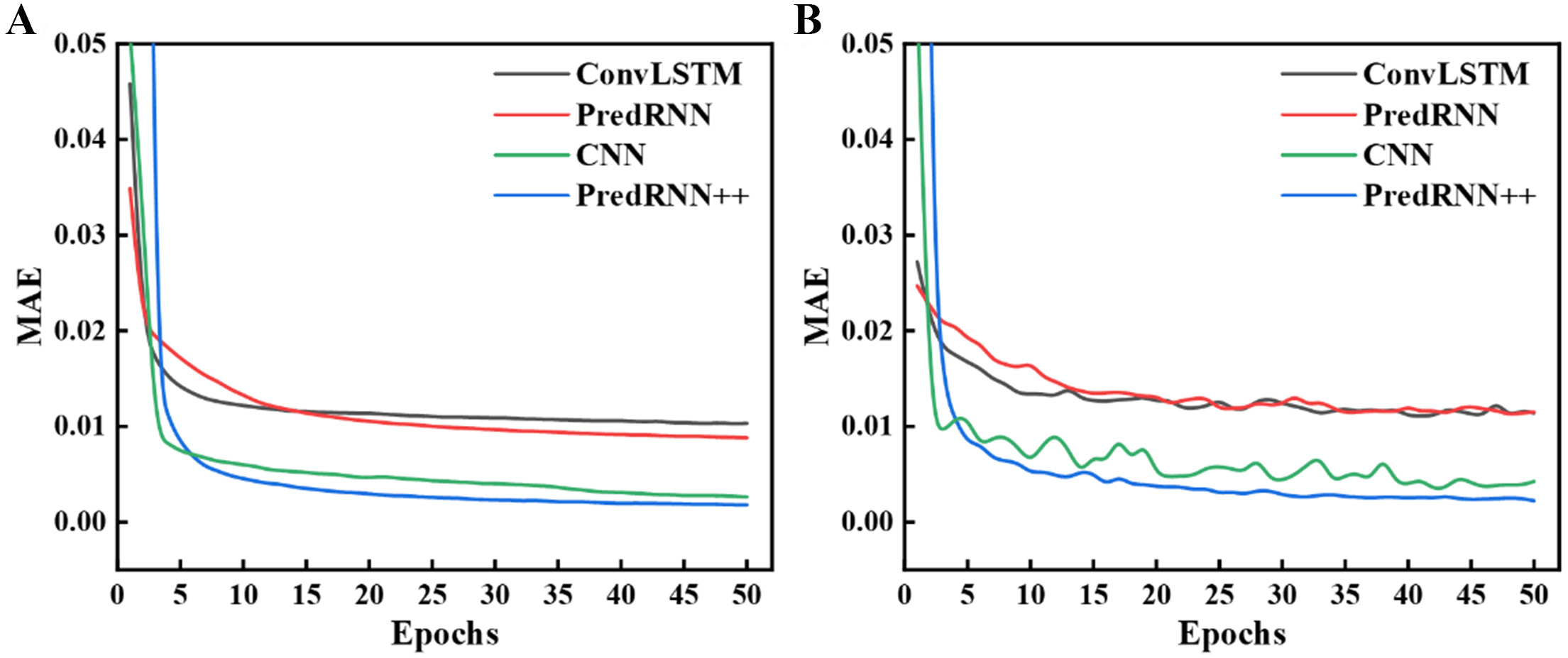
Figure 2. The MAE loss curves for different models after model parameter adjustment, (A) training set, (B) testing set. MAE: Mean absolute error; ConvLSTM: convolutional long short-term memory; PredRNN: predictive recurrent neural network; CNN: convolutional neural network; PredRNN++: predictive recurrent neural network++.
The trained model is used for subsequent microstructure prediction to assess its extrapolation capability. Figure 3 and Figure 4 show the relationships between structural similarity (SSIM) and predicted step for each model in the training set and testing set, respectively. As the predicted step increases, the SSIM decreases and the error increases. The predicted step is the number of step forward in the deep learning model based on the input data. For example, if the input data is t5- t9 and the predicted step is 25, the output data will be t34. The predicted step interval corresponds to the time step interval in PF simulations. The PredRNN model exhibits slight differences, it performs better at 6-12 predicted steps. This is because its model framework is more suitable for mid-term predictions. However, for long-term predictions, the model’s limited capabilities still lead to higher errors. As shown in Figure 3, in the training set, the PredRNN model only achieves SSIM values comparable to the PredRNN++ model at 28 and 30 predicted steps. Conversely, as shown in Figure 4, on the testing set, the PredRNN model consistently yields lower average SSIM values than the PredRNN++ model at every predicted step. At the 30 predicted step, the average SSIM value of the PredRNN model on the testing set is 0.879, while the average SSIM value of the PredRNN++ model on the testing set is 0.914. This indicates that the PredRNN++ model demonstrates superior generalization capabilities compared to the PredRNN model. The ConvLSTM model performs the worst in the four models, as it only contains the convolutional LSTM model[57], has a simple framework, lacks of extrapolation capability, and exhibits distorted predictions. The CNN model performs well on the training set. But on the testing set, as the number of predicted steps increases, the SSIM rapidly decreases, indicating that the CNN model’s extrapolation capability is limited and unsuitable for long-term predictions.
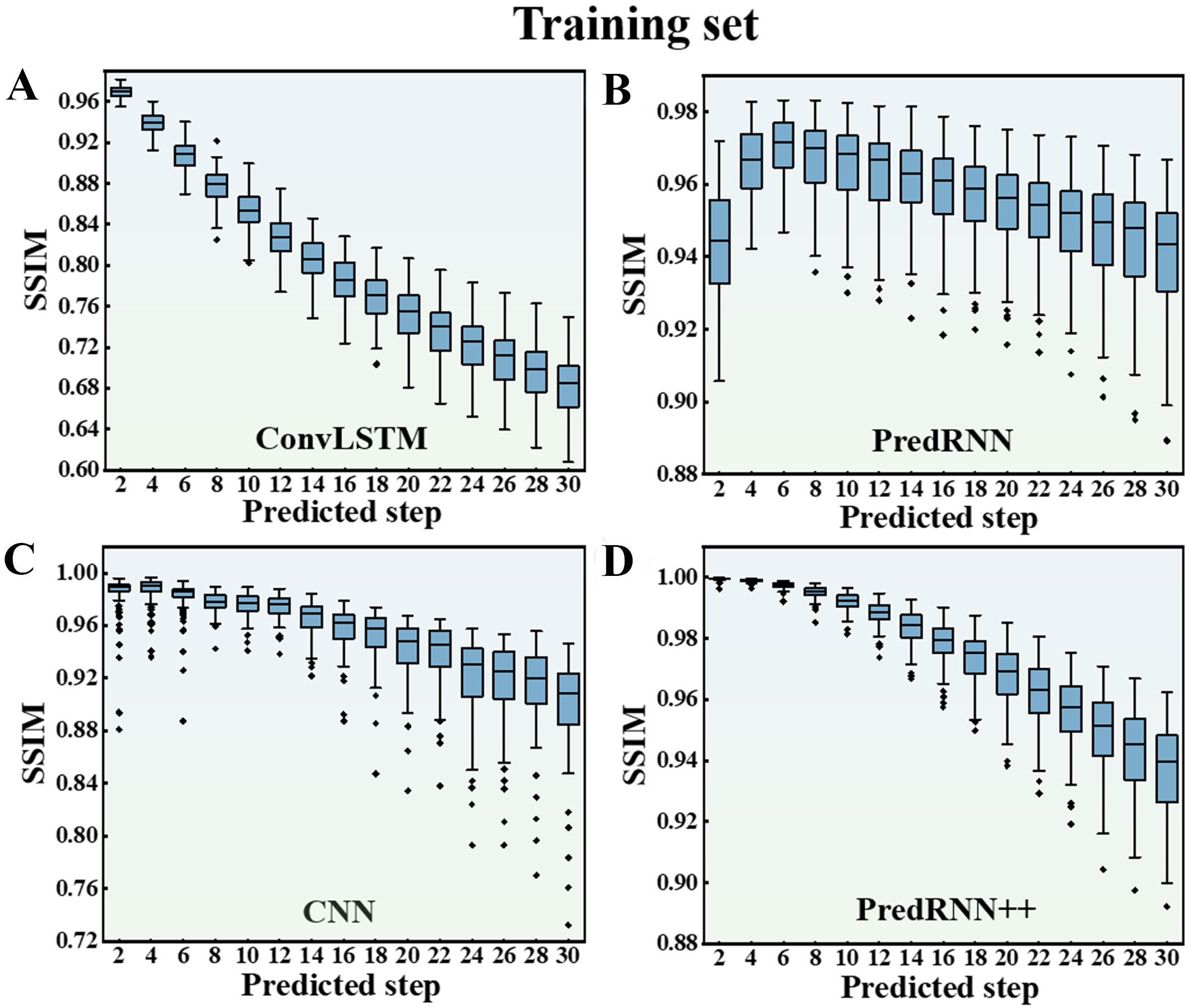
Figure 3. The distribution of structural similarity of different models with predicted steps in the training set, (A) ConvLSTM, (B) PredRNN, (C) CNN, (D) PredRNN++. ConvLSTM: Convolutional long short-term memory; PredRNN: predictive recurrent neural network; CNN: convolutional neural network; PredRNN++: predictive recurrent neural network++; SSIM: structural similarity.
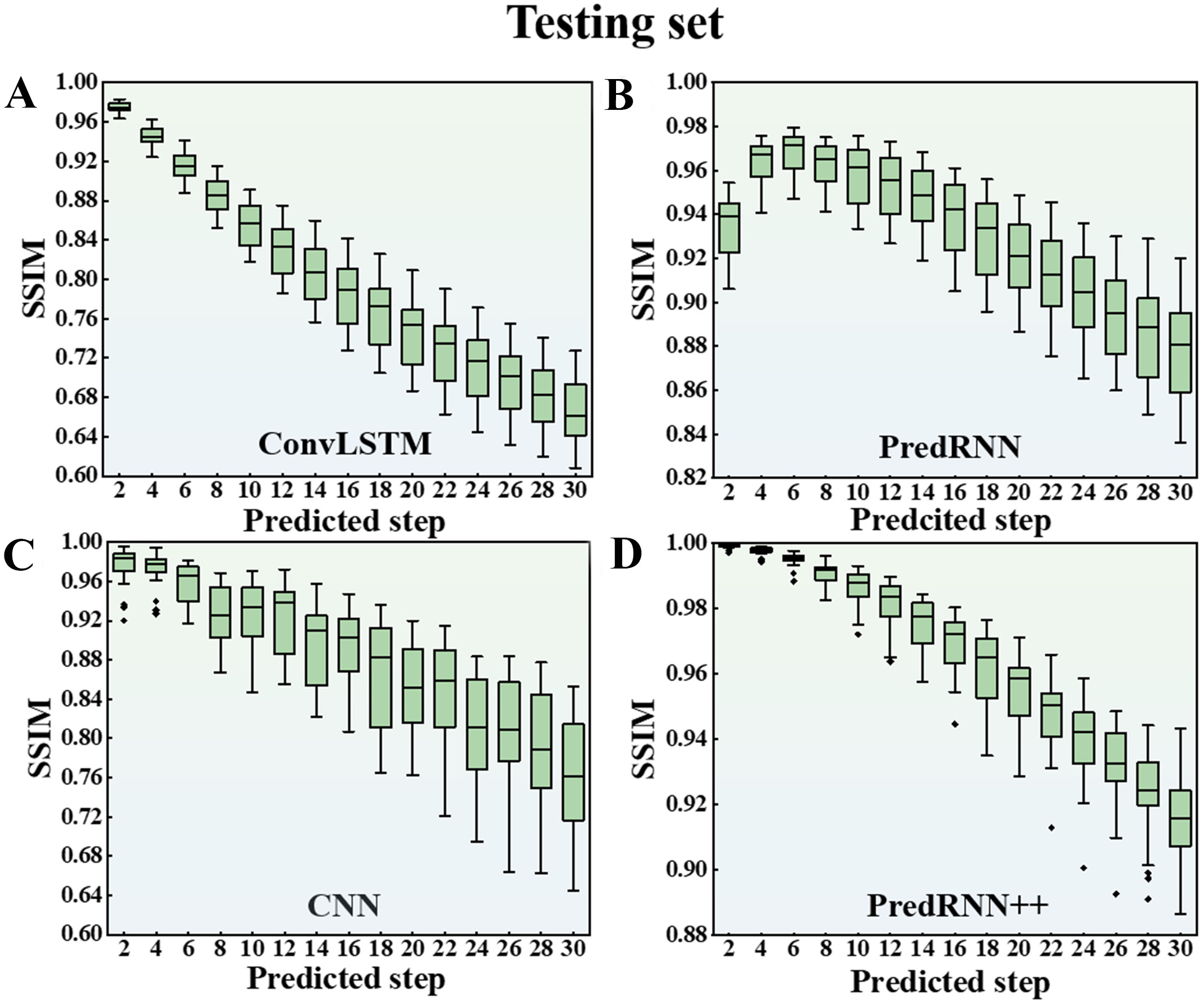
Figure 4. The distribution of the structural similarity of different models with predicted steps in the testing set, (A) ConvLSTM, (B) PredRNN, (C) CNN, (D) PredRNN++. ConvLSTM: Convolutional long short-term memory; PredRNN: predictive recurrent neural network; CNN: convolutional neural network; PredRNN++: predictive recurrent neural network++; SSIM: structural similarity.
Although the convolutional model has sufficient complexity and good extrapolation performance on the training set, its computational method is not suitable for subsequent predictions involving time-series feature data, leading to significant errors in unknown data spaces. The PredRNN++ model integrates the Causal LSTM and GHU frameworks[53]. The Causal LSTM framework has the cascaded dual-storage operation to compute temporal and spatial memory streams separately, thereby avoiding temporal-spatial memory-forgetting conflicts. The GHU framework adaptively regulates long-term and short-term frame relationships to enable recursive information propagation, mitigating the vanishing gradient problem in long-term predictions. Although errors gradually increase, the model maintains a high level of structural similarity. In summary, compared with other common time series prediction models, the PredRNN++ model has significant advantages in long-term prediction of the aging microstructure of superalloys.
In addition to the data of precipitation microstructure of superalloys used in this study, we also used the data of another microstructure through spinodal decomposition data[58] for PredRNN++ model training. Using the evaluation metrics employed in their proposed model [root mean square error (RMSE) and SSIM], the advantages of the PredRNN++ model are demonstrated. With the first 10 steps of PF microstructure data as input to predict the subsequent 200 steps, the model underwent 100 training iterations. Figure 5 demonstrates the performance capability of the PredRNN++ model. It is found that when predicting the first 50 steps of microstructural evolution, the SSIM value exceeds 0.99 and the RMSE is less than 0.019. Furthermore, when the predicted step is 200, the SSIM reaches 0.82 and the RMSE is 0.148. These results outperform the model proposed by Yang et al.[58]. The PredRNN++ model is not only applicable to complex multi-field microstructure prediction, but also has superior performance in single-field microstructure prediction.
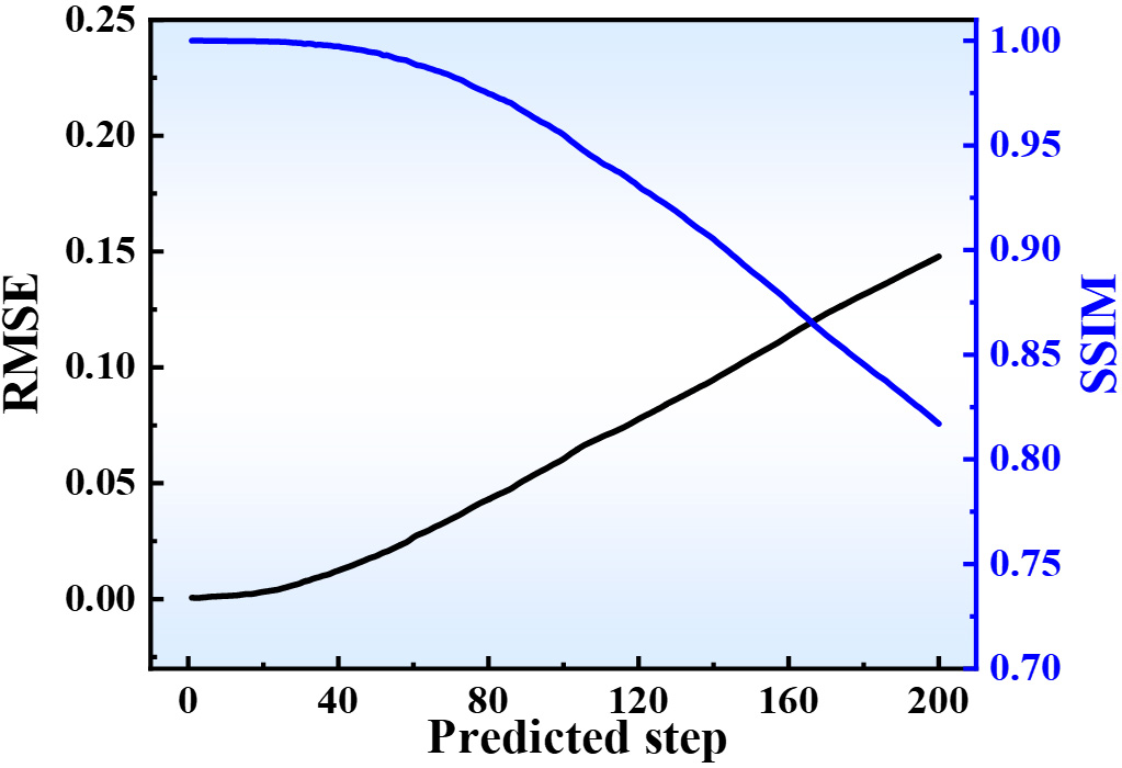
Figure 5. PredRNN++ predictions of spinodal decomposition based on the data of first 10 input steps. PredRNN++: Predictive recurrent neural network++; RMSE: root mean square error; SSIM: structural similarity.
Model performance evaluation of PredRNN++ model
Optimal parameters are used to further investigate the model’s performance across different output steps in the PredRNN++ model. The optimal parameters are as follows: filter = (64, 64, 64), kernel function = (5, 5, 5), number of cells = 3, optimizer = Adam, and learning rate = 0.0005. The process of determining hyperparameters is illustrated in Supplementary Figure 3.
To test the effects of predicted step on the errors of PredRNN++ model. Figure 6 shows the learning curves for different predicted steps. The MAE error increases with the number of predicted steps. When the predicted step is 15, the error curve fluctuates significantly and does not converge. When the predicted step is 10, the final error on the testing set is 0.006, while it is 0.0017 when the predicted step is 5, which is less than 50% of the former.
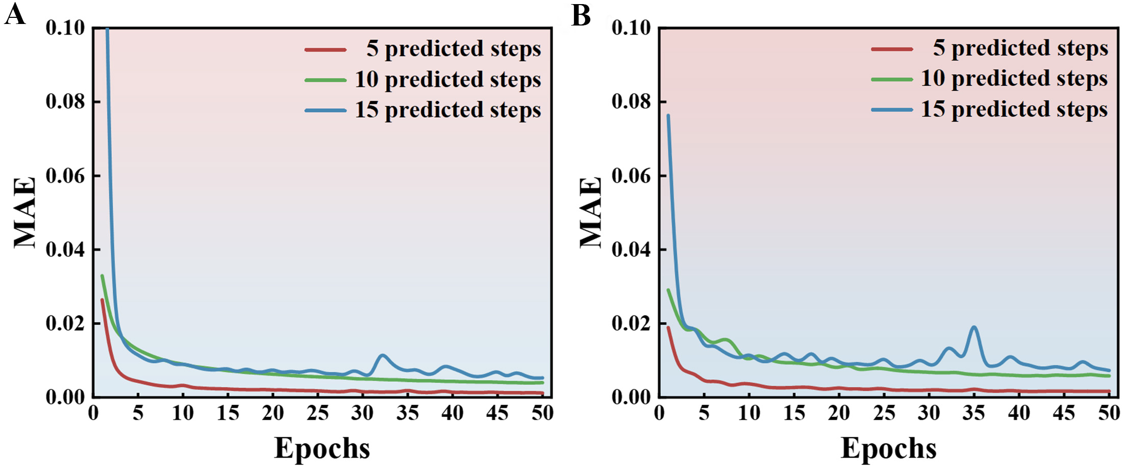
Figure 6. The MAE loss curves of different predicted steps of the PredRNN++ model, (A) training set, (B) testing set. MAE: Mean absolute error; PredRNN++: predictive recurrent neural network++.
Figure 7 shows the error performance of the PredRNN++ model when different input steps are used. When the initial input is the later-stage microstructure data, the PredRNN++ model performs better, with lower error and variance. This is because the later stage precipitates have a more stable microstructure, with fewer interface locations experiencing unexpected fluctuations. After training, the PredRNN++ model provides more stable predictions of precipitation microstructural evolution. Especially when the input step is in the range of t13-t17 and the predicted step is 25, the final SSIM of t42 remains at 0.96, and the MAE is 0.0047. It indicates that when the initial input is in the mid-stage of PF results, the PredRNN++ model can directly predict the long-time evolution process and maintain a small error. In other words, the PredRNN++ model can directly reduce the time required for PF computation by 50%.
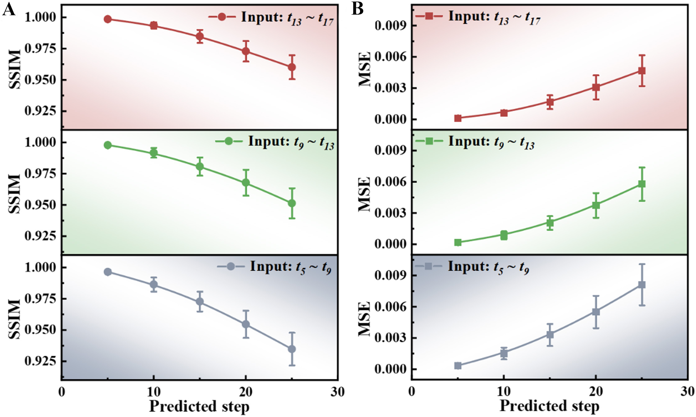
Figure 7. Error performance of the PredRNN++ model at different initial input steps, (A) SSIM, (B) MSE. PredRNN++: Predictive recurrent neural network++; SSIM: structural similarity; MSE: mean square error.
Figure 8 shows the results of the PredRNN++ model at different predicted steps when the input data is t5-t9. Where the errors are concentrated at the boundaries of precipitates. When the predicted count is less than 5 steps, the model can accurately predict the precipitation process with almost no error. When the predicted time is long and exceeds 13 steps, errors at the precipitation boundaries emerge. However, the overall precipitation is still similar to the PF microstructure, enabling the identification of local coarsening connections and dissolved precipitates. To check the component conservation through iterative loop, we examined the overall components change with the time steps, as shown in Supplementary Figure 4. In where, when the predicted step less than 10, the component deviation of Al is smaller than 0.02 (at.%), as the predicted step increases to 20, the average component deviation is 0.16 (at.%), at the same time, the morphological deviation becomes obvious [Figure 8, t18-t22]. Due to the uniform data-processing method, this increase is negligible within the component field when controlling the predicted steps. The training error of the deep learning model exerts a greater influence on morphology.
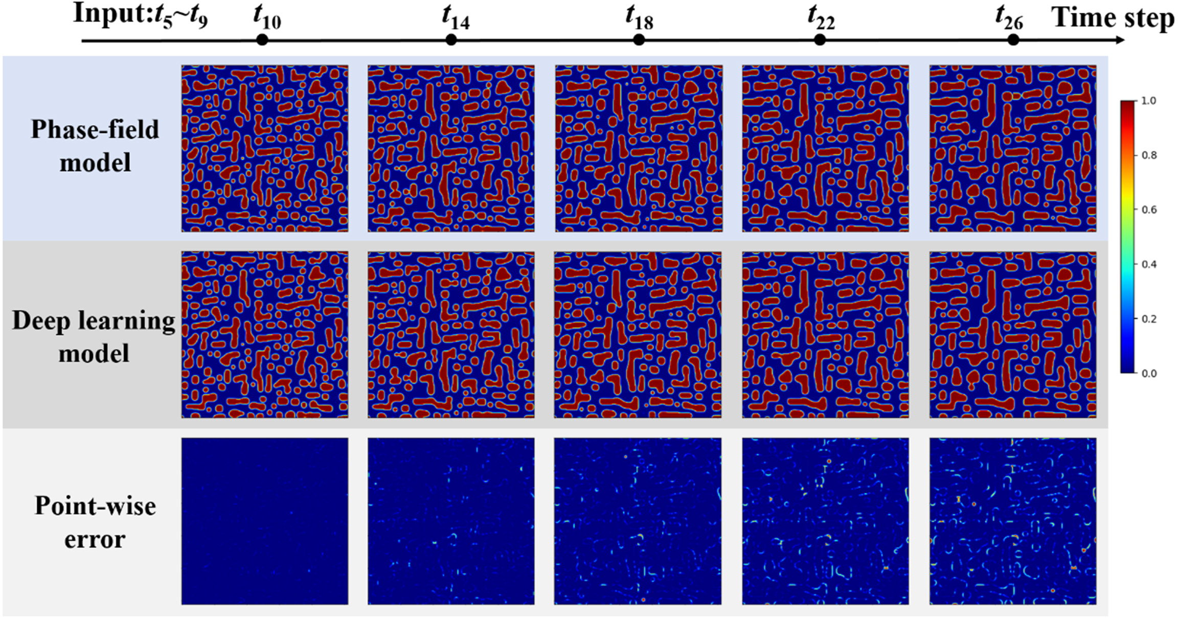
Figure 8. Predicted microstructural evolution of PredRNN++ model by using the PF input microstructure data of step t5-t9 with Ni-15.9Al (at.%) superalloy. PredRNN++: Predictive recurrent neural network++; PF: phase-field.
Accelerated PF simulation
To fully leverage the advantages of deep learning models, we propose a hybrid acceleration strategy. Figure 9 illustrates the schematic diagram of accelerated PF simulation by alternating PF model and deep learning model in computation. In which, the PF model performs initial simulations to adjust and obtain the proper precipitate microstructure, followed by the deep learning model for rapid prediction to reduce computation time. Through this iterative operation, the hybrid acceleration strategy achieves accurate evolution of precipitation microstructure while significantly reducing computational time. The iterative loop we designed involves the PF running n steps, while the PredRNN++ model runs 2n steps. This decision is based on the performance characteristics of the PredRNN++ model. When predicting the subsequent 2n steps based on n input data, the PredRNN++ model demonstrates controllable distortion. Incorporating it into the PF model does not introduce notable differences.
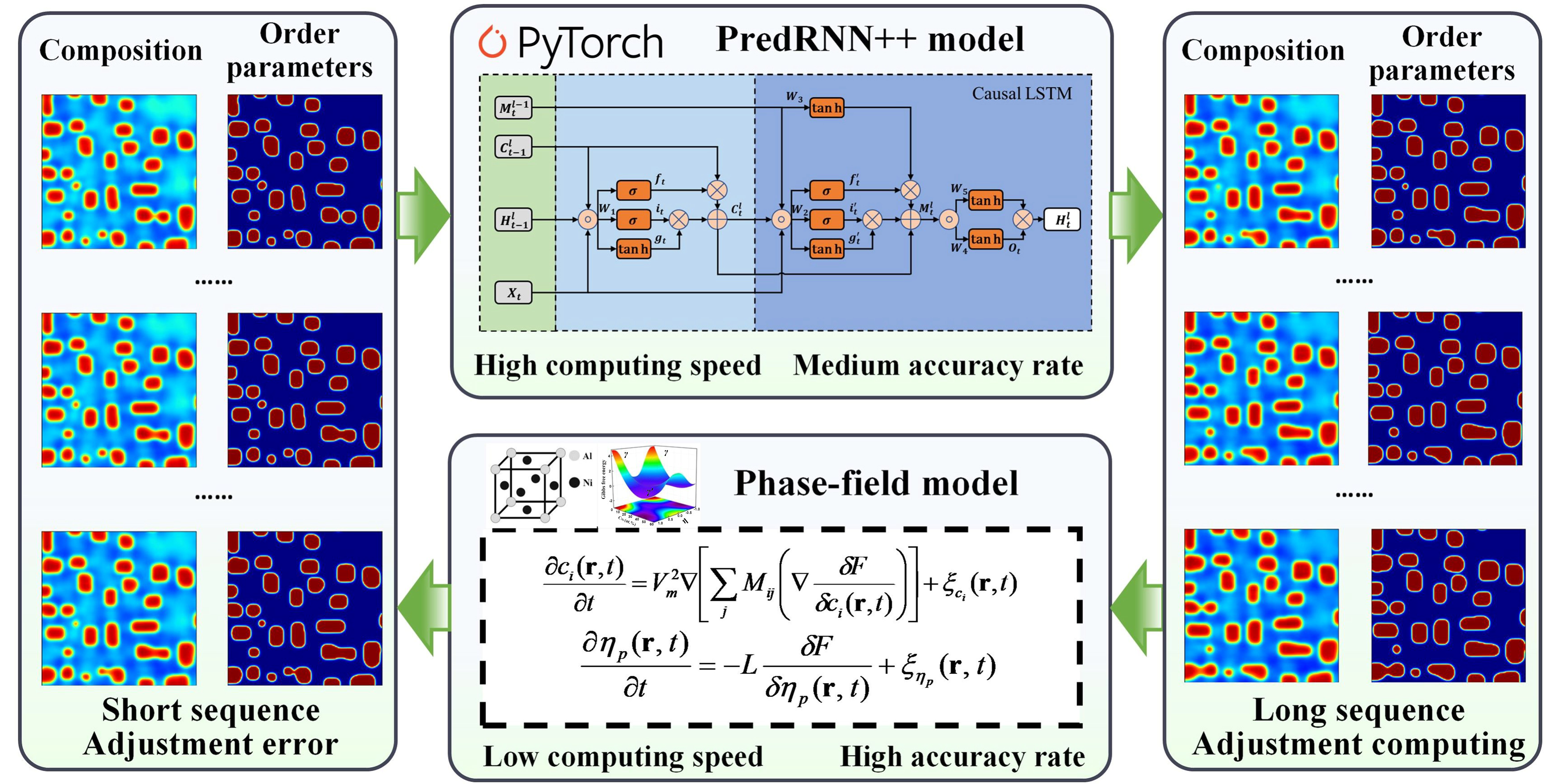
Figure 9. Schematic diagram of accelerated PF simulation by PredRNN++ model. PF: Phase-field; PredRNN++: predictive recurrent neural network++.
Figure 10 shows the performance results of the hybrid computation of the integrated PredRNN++ and PF model. For the initial PF precipitation microstructure at 40 min of t10, the PredRNN++ model is used to compute and predict for the next 10 steps to t20, then the PF simulation is performed based on the PredRNN++ predicted microstructure and handles for the next 5 steps to t25, and so on. This alternative calculation can be processed when a threshold error occurs. Compared to the 160 min consumed by PF from t10 to t50, the hybrid model reduces the computation time to only 43 min, maintaining the MSE error within 0.004 and achieving 3.7 times improvement in efficiency. It should be noted that the PredRNN++ prediction in 1 min/10 step will consume the PF 40 min/10 step, so the velocity of PredRNN++ is 40 times that of PF. Compared to the deep learning model, the hybrid model, including the alternate PF simulation, with the materials’ physical information adjusted in the PredRNN++ prediction, significantly reduces the rate of error increase. The error at t50 obtained by the hybrid model is close to that at the 17 predicted step of the single PredRNN++ model shown in Figure 8. The hybrid model can accurately identify the coarsening or dissolution of the precipitated phase.
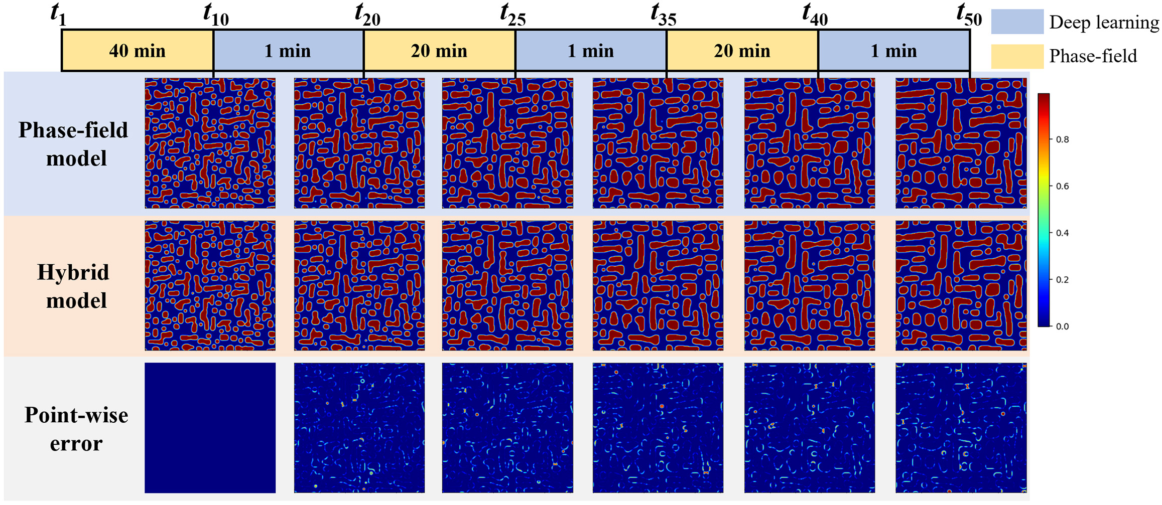
Figure 10. The performance of the hybrid model prediction on microstructural evolution of Ni-15.9Al (at.%) superalloy at 873 K with the PredRNN++ and PF simulation. PredRNN++: Predictive recurrent neural network++; PF: phase-field.
Figure 11 compares the different morphologies obtained from the hybrid model and the PF simulation. The hybrid model’s predictions show higher accuracy within the precipitated phase. The errors are minor and occur only at the boundaries between the precipitated and matrix phases, indicating that the hybrid model can maintain high fidelity in the morphology image across different shapes.
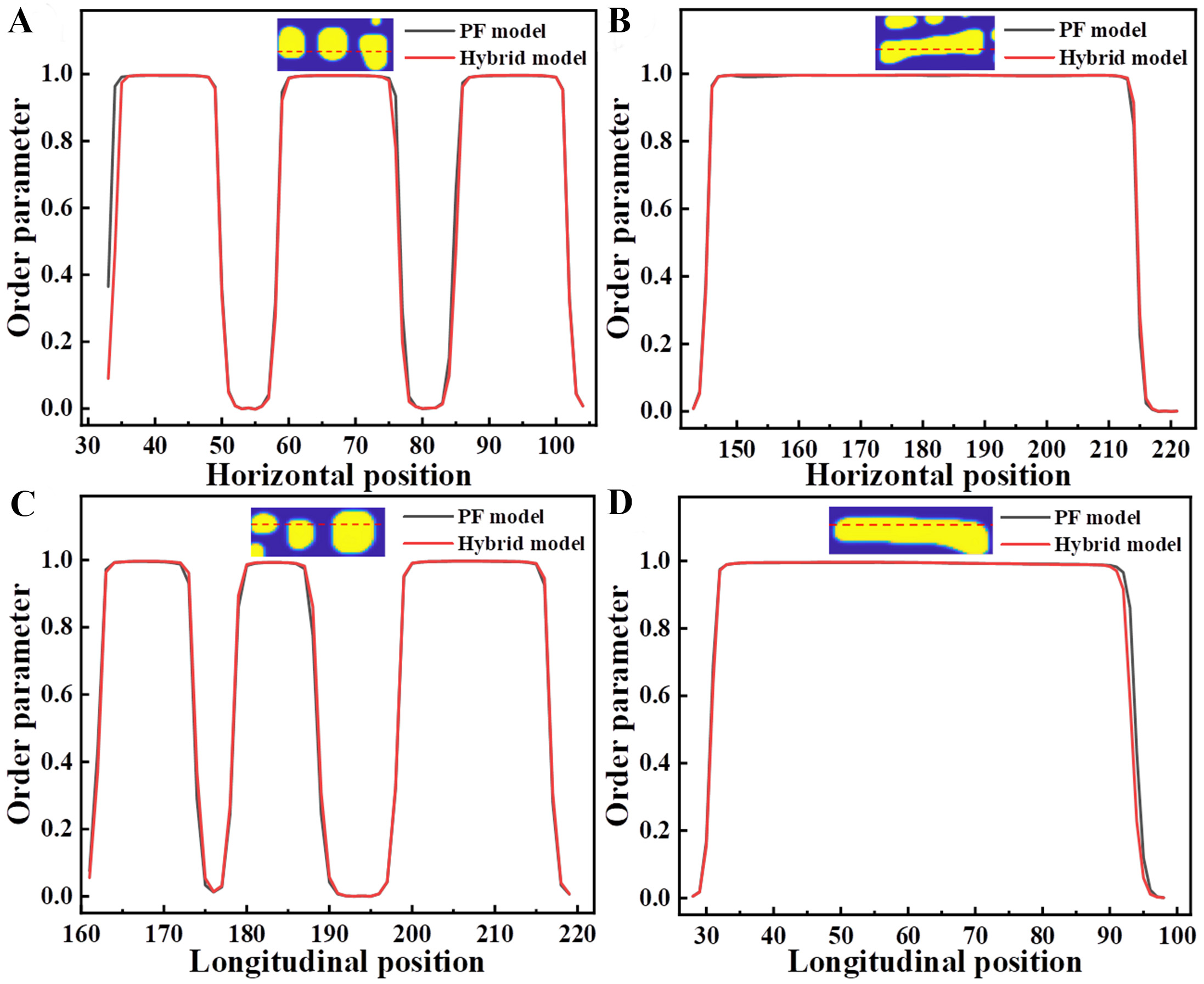
Figure 11. Comparison of Ni-15.9Al (at.%) superalloy order parameters predicated by the hybrid model and PF model for different morphologies, (A) horizontal separated particles, (B) horizontal coalescent particles, (C) longitudinal separated particles, (D) longitudinal coalescent particles. PF: Phase-field.
PredRNN++ performance for different morphologies
To elaborate on the predictive ability of the PredRNN++ model for the microstructural evolution, the model was trained using data from different shapes of the precipitated phase. The microstructure of precipitated phase of the Ni-Al superalloys exhibits both square and circular shapes, referred to as the mixed-shape. For different shaped precipitated phases, the hyperparameters of the retrained PredRNN++ model are consistent with those of the Ni-Al superalloys. The parameters were not modified to enhance comparability. The model training results are shown in Supplementary Figure 5. In the Co-based superalloy, precipitated phase with cubic shape is adopted, the microstructure data of Co-10Al-10W (at.%) superalloy with six sets of lattice mismatches are used as the cubic microstructure data source. The specific data are provided in Supplementary Table 3. Supplementary Figure 6 shows the microstructure prediction of the PredRNN++ model for the Co-based superalloy Co-10Al-10W (at.%). It can be seen that the PredRNN++ model performs worse in predicting cubic precipitates. When the time step is t39, the PF microstructure exhibits a good cubic shape, while the microstructure of the hybrid model shows a non-cubic shape, with some regions still no precipitates, this means the precipitation lag for deep learning prediction.
Figure 12 shows the performance of the hybrid model for the precipitation prediction in Co-10Al-10W (at.%) superalloy. Where the initial microstructure is simulated by PF for 180 min at t23, then the PredRNN++ prediction for 1 min/16 step, and PF simulation for 60 min/8 step, to the next time of t47, and so on. The error occurred at the boundaries of precipitates, as shown by the point-wise error at t119. Especially, some smaller precipitated phases do not dissolve and disappear in the hybrid model, while coarsening and growing, as labelled by the green circle. The results indicate that the sharp boundaries of cubic precipitates may be misidentified by the PredRNN++ model, especially during coarsening and dissolution of small particles. This means the physical properties of the microstructural evolution can be misidentified. It is noting that the predicted step is prolonged in this case, for PredRNN++ prediction acceleration is 120 times of PF, which is much higher than 40 times of Figure 10. Therefore, the PredRNN++ model shows some limited predictive capability for the sharp interface transition and is more capable for the smooth interface of particle growth and coarsening.
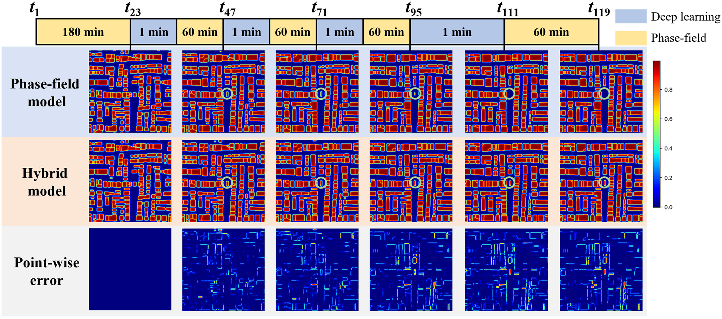
Figure 12. The performance of the hybrid model prediction on microstructural evolution of Co-10Al-10W (at.%) superalloy at 1,173 K with the PredRNN++ and PF simulation. PredRNN++: Predictive recurrent neural network++; PF: phase-field.
Next, the near circular shaped precipitates are predicated by using the aging microstructure of Ni-10Al-8.5Cr-2Ta (at.%) superalloy. The aging microstructural evolution of Ni-10Al-8.5Cr-2Ta (at.%) with different interfacial energy coefficients and lattice mismatches is used as the circular data source. The specific data are provided in Supplementary Table 4. Supplementary Figure 7 shows the microstructure prediction of PredRNN++ model for Ni-10Al-8.5Cr-2Ta (at.%). It can be seen that the PredRNN++ model performs well in predicting circular shapes. For morphologies predicted within 13 predicted step, the MAE error is less than 0.009. When the predicted step reaches 17, a small error occurs at the coarsened connection points, with the MAE value of 0.011. The PredRNN++ model performs well in predicting the smooth particle growth.
Figure 13 shows the performance of hybrid model for the microstructure of Ni-10Al-8.5Cr-2Ta (at.%) superalloy. Where the initial microstructure is simulated by PF for 120 min at t20, then the PredRNN++ prediction for 1 min/15 step, and alternate PF simulation for 30 min/5 step, to the next time of t40, and so on. It is found that the errors in the hybrid model are concentrated at the coalescence points of precipitates, which is due to the tendency of the trained PredRNN++ model during the coarsening stage, as seen in Supplementary Figure 8 at t17. However, the overall error is relatively small, outperforming the cubic precipitates. Also, the PredRNN++ prediction acceleration is 90 times of PF in this case, which is higher than 40 times of Figure 10.
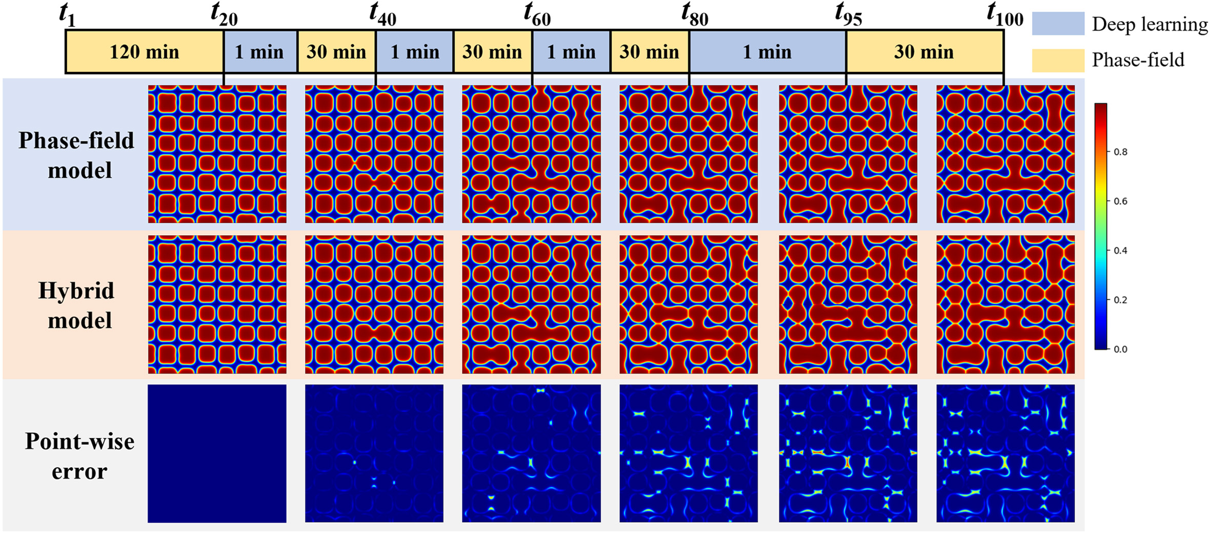
Figure 13. The performance of the hybrid model prediction on microstructure of Ni-10Al-8.5Cr-2Ta (at.%) superalloy at 1,073 K with the PredRNN++ and PF simulation. PredRNN++: Predictive recurrent neural network++; PF: phase-field.
Figure 14 shows the statistical correlation errors of the PredRNN++ model for different microstructure predictions. As shown in Figure 14A and B, among the numerical errors, the circular error is the smallest, followed by the mixed-shaped error, while the cubic error is the worst. The PredRNN++ model is suitable for predicting the growth and evolution process of circular precipitates.
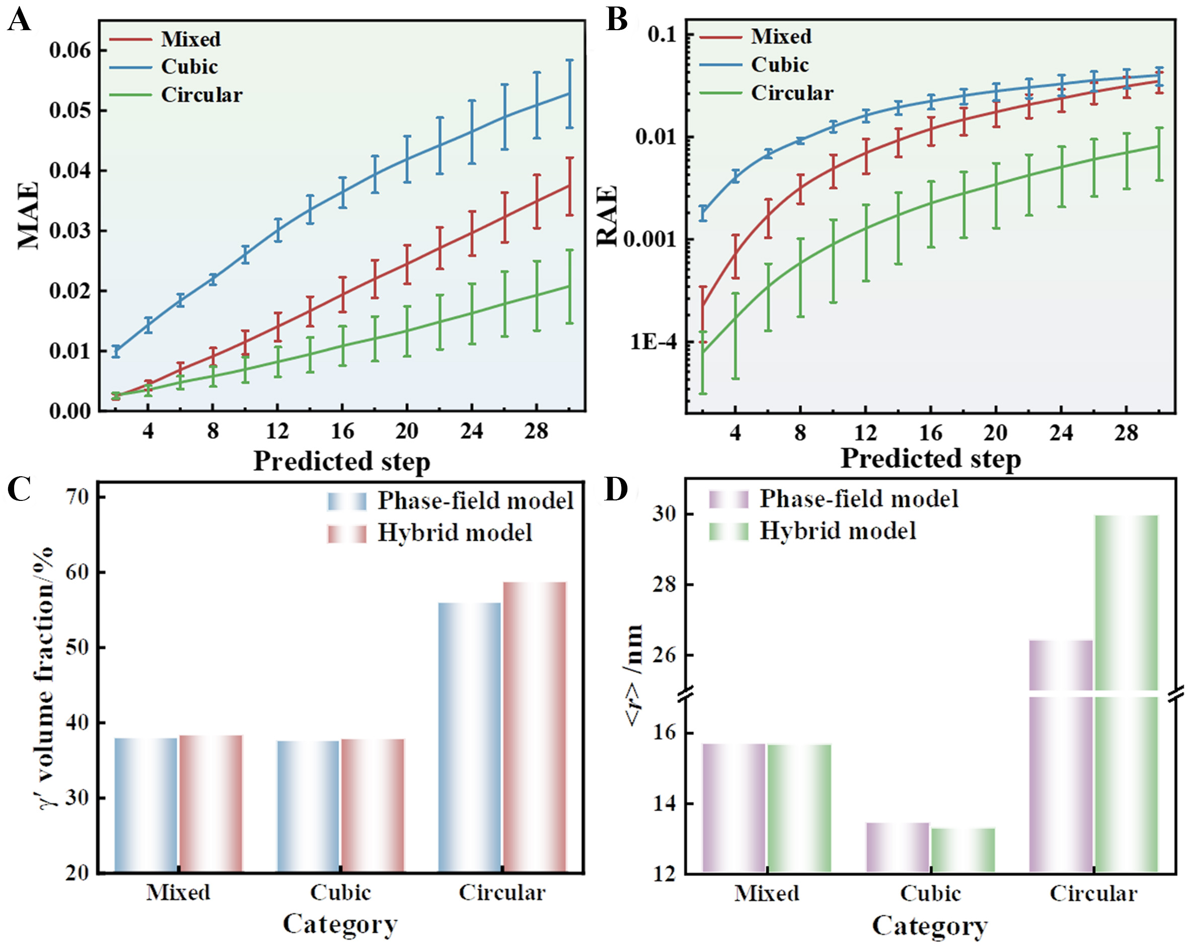
Figure 14. The PredRNN++ model performance of different morphologies comparison, (A) MAE for PredRNN++ model, (B) relative error (RAE) for PredRNN++ model, (C) γ′ volume fraction for hybrid model, (D) average radius for hybrid model. PredRNN++: Predictive recurrent neural network++; MAE: mean absolute error.
Supplementary Figure 8 shows the distribution of Al composition predicted by the PredRNN++ model at the predicted step of 20. As indicated in Supplementary Figure 8A and C, although the PredRNN++ model exhibits significant deviations in microstructure morphology and composition distribution when predicting Ni-15.9Al (at.%) and Ni-10Al-8.5Cr-2Ta (at.%) superalloys, the interface width remains largely unchanged, consistent with actual observations. In contrast, the interface width in Supplementary Figure 8 for Co-10Al-10W (at.%) exhibits changes, which is one of the factors influencing the formation of cubic precipitation phase particles.
Table 1 shows the prediction error of precipitation microstructure and overall acceleration efficiency obtained from the hybrid model. The mixed-shaped morphologies have the minimum MAE of 0.024. The computational efficiency of hybrid model of PredRNN++ and PF all exceeds 2.9 times that of the single PF model, for circular shape achieving an efficiency of 3.9 times.
Final error and overall acceleration efficiency obtained from the hybrid model for different shape of precipitates using all data set
| Source | Mixed | Cubic | Circular |
| MAE | 0.0240 ± 0.008 | 0.0486 ± 0.020 | 0.0288 ± 0.013 |
| Efficiency | 3.70 ± 0.09 | 2.90 ± 0.06 | 3.90 ± 0.10 |
In the quantitative microstructure analysis, Figure 14C and D show the comparison between the hybrid model and the PF simulation in terms of the volume fraction and the average particle radius of precipitates. The volume fraction and average particle radius of circular morphology obtained from the hybrid model have some differences from the PF values, as the hybrid model exhibits excessive coarsening. The predicted volume fraction and radius of mixed and cubic precipitates are almost the same for the hybrid model and the PF simulation. In all, the hybrid model exhibits smaller errors in numerical and microstructure analysis, and can accurately determine the growth and dissolution processes of the precipitated phase.
In addition to the common numerical comparisons, the statistical comparison method was employed to quantitatively analyze microstructural features derived from hybrid models and PF simulations using autocorrelation functions. The autocorrelation function extracts spatial structural features by discretizing the microstructure. The average radial autocorrelation function S(r) is calculated as the potential spatial description of particles. The comparison results of the hybrid model and the PF model are calculated based on the average feature size (AFSE) of the microstructure, as shown in Equation (24), to evaluate the prediction accuracy of the hybrid model[46].
Where rtrue and rpredict represent the radial average values obtained from the PF and the hybrid model, respectively.
The statistical errors of different shapes are shown in Figure 15. For the mixed shape, the mixed model shows the radial average microstructure parameter within the radial radius from r = 0 to 180 is similar to the simulation result of PF, and the overall AFSE is 2.36%. In the simulation of the cubic shape, when the radial distance is within r = 40, there is an obvious deviation between the model prediction and the PF result. Although the variations are both consistent with the radial distance increases, the overall AFSE still reaches 7.68%, indicating that the microstructure evolution under the cubic shape is not fully described in the model. The hybrid model predictions for circular morphologies exhibit high consistency with PF simulation results. With an overall AFSE as low as 1.38%, the model demonstrates high accuracy in numerically simulating circular shape.
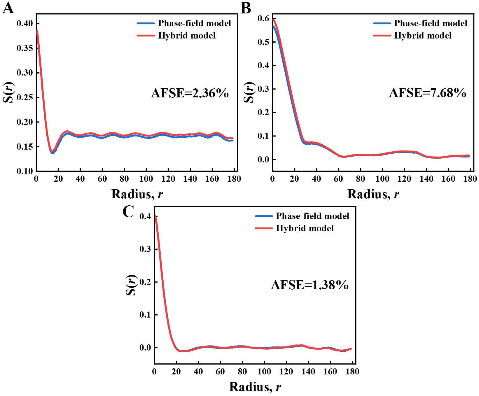
Figure 15. Comparison of the radial average of microstructure autocorrelation function S(r) for different morphologies in hybrid model (red) and the PF model (blue), (A) mixed shape, (B) cubic shape, (C) circular shape. PF: Phase-field; AFSE: average feature size.
Although the PredRNN++ model has the smallest error for predicting circular precipitates, the mixed-shape performs best overall. The prediction of both square and circular precipitates shows good performance, and the hybrid model can be used for quantitative analysis of precipitation kinetics for the mixed-shape. The prediction on abrupt interface evolution still needs optimization for the PredRNN++ model.
In conclusion, the PredRNN++ model was trained to predict the spatiotemporal evolution of precipitates in superalloys. The model’s capability is demonstrated through the precipitation evolution of different phase morphologies. This model can accurately predict twice or more of the subsequent evolutionary morphologies with minimal input data, while adapting to time-sensitive evolutionary rules across various situations. The PredRNN++ model can be applied to make preliminary predictions about the evolution of unknown morphologies. Additionally, the constructed hybrid model can be used to some extent for precipitation kinetics analysis of superalloys, and can be further optimized by incorporating physical constraints[59]. The PredRNN++ model is a purely data-driven deep learning model that can use the PDEs as a soft constraint for the loss function to enhance model accuracy. By expanding different data sources and assimilating the limited number of high-fidelity experimental image data into the model[60,61], the model’s generalization capability can be further improved.
CONCLUSIONS
In this study, we developed the PredRNN++ model to predict precipitation evolution in superalloys during aging processes. The PredRNN++ model, combining causal LSTM and GHU modules, demonstrates superior predictive performance. It can directly predict the subsequent evolution process using mid-term evolution data, thereby reducing PF computation time by 50%. The hybrid model integrating PredRNN++ model and PF simulation was developed for iterative computation, achieving computational efficiency at least 2.9 times higher than single PF models. This research accelerates the prediction of material evolution processes, opening an efficient computational pathway for discovering and understanding microstructural evolution. Additionally, the PredRNN++ model requires further optimization by incorporating physical information to ensure the conservation of component fields and achieve higher prediction accuracy.
DECLARATIONS
Authors’ contributions
Writing-original draft: Song, J.; Wang, S.
Conceptualization: Li, Y.
Writing-review & editing: Li, Y.
Validation and Visualization: Wang, S.; Zhang, Z.; Niu, K.
Data curation and Formal analysis: Wang, S.; Shan, Y.
All authors read and approved the final manuscript.
Availability of data and materials
Some results for supporting the study are given in the Supplementary Materials. Other raw data that support the findings of this study are available from the corresponding author upon reasonable request.
AI and AI-assisted tools statement
Not applicable.
Financial support and sponsorship
This work was supported by the National Natural Science Foundation of China (Grant No. 52275342).
Conflicts of interest
All authors declared that there are no conflicts of interest.
Ethical approval and consent to participate
Not applicable.
Consent for publication
Not applicable.
Copyright
© The Author(s) 2026.
Supplementary Materials
REFERENCES
1. Chen, L.; Zhao, Y. From classical thermodynamics to phase-field method. Prog. Mater. Sci. 2022, 124, 100868.
2. Zhao, Y. Understanding and design of metallic alloys guided by phase-field simulations. npj. Comput. Mater. 2023, 9, 94.
3. Mancias, J.; Vela, B.; Flórez-coronel, J.; et al. Mapping of microstructure transitions during rapid alloy solidification using Bayesian-guided phase-field simulations. Acta. Mater. 2025, 297, 121354.
4. Tang, Y.; Zhang, A.; Liu, H.; et al. Insight into scale selection of dimensionless phase-field model of alloy solidification. Mater. Des. 2025, 254, 114028.
5. Blixt, K. H.; Hallberg, H. Phase field crystal modeling of grain boundary migration: mobility, energy and structural variability. Acta. Mater. 2025, 297, 121318.
6. Jiang, L.; Liu, G.; Jin, P.; Shen, Y.; Wang, J. The driving force for twin boundary migration in phase field model coupled to crystal plasticity finite element. Int. J. Plast. 2025, 191, 104397.
7. Hu, J.; Xu, B.; Xiong, J.; Yu, C.; Kang, G. Deformation mechanism of non-textured and basal-textured polycrystalline Mg alloys: a coupled crystal plasticity-twinning phase field simulation. Int. J. Plast. 2025, 188, 104312.
8. Chen, J.; Guo, M.; Yang, M.; Cui, T.; Cui, B.; Zhang, J. Insight into element segregation mechanisms during creep in γʹ-strengthened Co-based superalloy by elastoplastic phase-field simulation. Prog. Nat. Sci. Mater. Int. 2024, 34, 873-9.
9. Zhang, H.; Zhang, Z.; Wang, S.; et al. Neutron irradiation and stress-induced creep rafting of α′ phase in Fe-Cr-Al alloy: crystal plasticity multi-phase-field simulation. J. Mater. Sci. Technol. 2026, 249, 164-73.
11. Allen, S. M.; Cahn, J. W. A correction to the ground state of FCC binary ordered alloys with first and second neighbor pairwise interactions. Scr. Metall. 1973, 7, 1261-4.
12. Doghman, J.; Bovet, C.; Ask, A. A finite element-based simulation of microstructure evolution through a 3D finite strain Cosserat phase-field model. Comput. Methods. Appl. Mech. Eng. 2025, 439, 117900.
13. Cao, W.; Yang, H.; Chen, W. An exponential time differencing Runge-Kutta method ETDRK32 for phase field models. J. Sci. Comput. 2024, 99, 6.
14. Krischok, A.; Yaraguntappa, B.; Keip, M. Fast implicit update schemes for Cahn-Hilliard-type gradient flow in the context of Fourier-spectral methods. Comput. Methods. Appl. Mech. Eng. 2024, 431, 117220.
15. Gültekin, O.; Dal, H.; Holzapfel, G. A. A phase-field approach to model fracture of arterial walls: theory and finite element analysis. Comput. Methods. Appl. Mech. Eng. 2016, 312, 542-66.
16. Valizadeh, N.; Zhuang, X.; Rabczuk, T. A monolithic finite element method for phase-field modeling of fully Eulerian fluid-structure interaction. Comput. Methods. Appl. Mech. Eng. 2025, 435, 117618.
17. Kristensen, P. K.; Martínez-pañeda, E. Phase field fracture modelling using quasi-Newton methods and a new adaptive step scheme. Theor. Appl. Fract. Mech. 2020, 107, 102446.
18. Liao, H.; Ji, B.; Zhang, L. An adaptive BDF2 implicit time-stepping method for the phase field crystal model. IMA. J. Numer. Anal. 2022, 42, 649-79.
19. Shi, X.; Huang, H.; Cao, G.; Ma, X. Accelerating large-scale phase-field simulations with GPU. AIP. Adv. 2017, 7, 105216.
20. Li, H.; Song, Z. A reduced-order finite element method based on proper orthogonal decomposition for the Allen-Cahn model. J. Math. Anal. Appl. 2021, 500, 125103.
21. Zhang, A.; Guo, Z.; Jiang, B.; Xiong, S.; Pan, F. Numerical solution to phase-field model of solidification: a review. Comput. Mater. Sci. 2023, 228, 112366.
22. Butler, K. T.; Davies, D. W.; Cartwright, H.; Isayev, O.; Walsh, A. Machine learning for molecular and materials science. Nature 2018, 559, 547-55.
23. He, Y.; De Breuck, P.; Weng, H.; Giantomassi, M.; Rignanese, G. Machine learning on multiple topological materials datasets. npj. Comput. Mater. 2025, 11, 181.
24. Li, K.; Rubungo, A. N.; Lei, X.; et al. Probing out-of-distribution generalization in machine learning for materials. Commun. Mater. 2025, 6, 9.
25. Tao, Q.; Yang, X.; Bao, L.; et al. Transforming machine learning model knowledge into material insights for multi-principal-element superalloy phase design. npj. Comput. Mater. 2025, 11, 99.
26. Barik, R. K.; Woods, L. M. Frictional properties of two-dimensional materials: data-driven machine learning predictive modeling. ACS. Appl. Mater. Interfaces. 2024, 16, 40149-59.
27. Qin, G.; Wei, Y.; Yu, L.; et al. Predicting lattice thermal conductivity from fundamental material properties using machine learning techniques. J. Mater. Chem. A. 2023, 11, 5801-10.
28. Kim, C.; Pilania, G.; Ramprasad, R. Machine learning assisted predictions of intrinsic dielectric breakdown strength of ABX3 perovskites. J. Phys. Chem. C. 2016, 120, 14575-80.
29. Dai, M.; Demirel, M. F.; Liang, Y.; Hu, J. Graph neural networks for an accurate and interpretable prediction of the properties of polycrystalline materials. npj. Comput. Mater. 2021, 7, 103.
30. Li, Z.; Hernández, F. J.; Salguero, C.; Lopez, S. A.; Crespo-otero, R.; Li, J. Machine learning photodynamics decode multiple singlet fission channels in pentacene crystal. Nat. Commun. 2025, 16, 1194.
31. Liao, W.; Yuan, R.; Xue, X.; Wang, J.; Li, J.; Lookman, T. Unsupervised learning-aided extrapolation for accelerated design of superalloys. npj. Comput. Mater. 2024, 10, 171.
32. Liu, P.; Huang, H.; Antonov, S.; et al. Machine learning assisted design of γ′-strengthened Co-base superalloys with multi-performance optimization. npj. Comput. Mater. 2020, 6, 62.
33. Deng, Y.; Zhang, Y.; Gong, X.; et al. An intelligent design for Ni-based superalloy based on machine learning and multi-objective optimization. Materials. &. Design. 2022, 221, 110935.
34. Ye, W.; Chen, C.; Wang, Z.; Chu, I.; Ong, S. P. Deep neural networks for accurate predictions of crystal stability. Nat. Commun. 2018, 9, 3800.
35. Azimi, S. M.; Britz, D.; Engstler, M.; Fritz, M.; Mücklich, F. Advanced steel microstructural classification by deep learning methods. Sci. Rep. 2018, 8, 2128.
36. Maiti, C.; Muthuswamy, S. Classification of materials in cylindrical workpieces using image processing and machine learning techniques. Int. J. Prod. Res. 2023, 62, 2566-83.
37. Cao, Y.; Zhang, C.; Tang, S.; et al. Machine learning to predict phase transformation products and their morphologies - application in design of lean high strength steel. Mater. Des. 2025, 258, 114642.
38. Lee, K.; Ayyasamy, M. V.; Delsa, P.; Hartnett, T. Q.; Balachandran, P. V. Phase classification of multi-principal element alloys via interpretable machine learning. npj. Comput. Mater. 2022, 8, 25.
39. Zhang, X.; Sun, J.; Zhang, Y.; et al. Machine learning for phase prediction of high entropy carbide ceramics from imbalanced data. npj. Comput. Mater. 2026, 12, 22.
40. Malashin, I.; Martysyuk, D. Powder particle classification with scanning electron microscopy images using machine learning techniques. Expert. Syst. Appl. 2025, 286, 128001.
41. He, J.; Zhou, Y.; Zhang, P.; Zhai, H. Machine learning assisted fast optical identification of 2D materials. Appl. Surf. Sci. 2025, 686, 162110.
42. Stan, T.; Thompson, Z. T.; Voorhees, P. W. Optimizing convolutional neural networks to perform semantic segmentation on large materials imaging datasets: X-ray tomography and serial sectioning. Mater. Charact. 2020, 160, 110119.
43. Dingreville, R.; Roberston, A. E.; Attari, V.; et al. Benchmarking machine learning strategies for phase-field problems. Modelling. Simul. Mater. Sci. Eng. 2024, 32, 065019.
44. Oommen, V.; Shukla, K.; Desai, S.; Dingreville, R.; Karniadakis, G. E. Rethinking materials simulations: blending direct numerical simulations with neural operators. npj. Comput. Mater. 2024, 10, 145.
45. Fetni, S.; Pham, T. Q. D.; Hoang, T. V.; et al. Capabilities of auto-encoders and principal component analysis of the reduction of microstructural images; application on the acceleration of phase-field simulations. Comput. Mater. Sci. 2023, 216, 111820.
46. Hu, C.; Martin, S.; Dingreville, R. Accelerating phase-field predictions via recurrent neural networks learning the microstructure evolution in latent space. Comput. Methods. Appl. Mech. Eng. 2022, 397, 115128.
47. Wu, P.; Iquebal, A. S.; Ankit, K. Emulating microstructural evolution during spinodal decomposition using a tensor decomposed convolutional and recurrent neural network. Comput. Mater. Sci. 2023, 224, 112187.
48. Ahmad, O.; Kumar, N.; Mukherjee, R.; Bhowmick, S. Accelerating microstructure modeling via machine learning: a method combining Autoencoder and ConvLSTM. Phys. Rev. Mater. 2023, 7, 083802.
49. Gesch, A.; Hu, C. Accelerating phase-field simulation of coupled microstructural evolution using autoencoder-based recurrent neural networks. J. Mater. Inf. 2025, 5.
50. Oommen, V.; Shukla, K.; Goswami, S.; Dingreville, R.; Karniadakis, G. E. Learning two-phase microstructure evolution using neural operators and autoencoder architectures. npj. Comput. Mater. 2022, 8, 190.
51. Teichert, G. H.; Garikipati, K. Machine learning materials physics: surrogate optimization and multi-fidelity algorithms predict precipitate morphology in an alternative to phase field dynamics. Comput. Methods. Appl. Mech. Eng. 2019, 344, 666-93.
52. Jokisaari, A.; Voorhees, P.; Guyer, J.; Warren, J.; Heinonen, O. Benchmark problems for numerical implementations of phase field models. Comput. Mater. Sci. 2017, 126, 139-51.
53. Wang, Y.; Gao, Z.; Long, M.; Wang, J.; Yu, P. S. PredRNN++: towards a resolution of the deep-in-time dilemma in spatiotemporal predictive learning. In International Conference on Machine Learning, Stockholm, Sweden, July 10-15, 2018; PMLR: 2018; Vol. 80, pp 5123-32. https://proceedings.mlr.press/v80/wang18b.html. (accessed 2026-05-21).
54. Wang, Y.; Long, M.; Wang, J.; Gao, Z.; Yu, P. S. PredRNN: Recurrent neural networks for predictive learning using spatiotemporal LSTMs. In Advances in Neural Information Processing Systems, Long Beach, CA, USA, December 4-9, 2017; Curran Associates, Inc.: Red Hook, NY, USA, 2017; Vol. 30, pp 879-88. https://proceedings.neurips.cc/paper/2017/hash/e. (accessed 2026-05-21).
55. Wang, Y.; Wu, H.; Zhang, J.; et al. PredRNN: a recurrent neural network for spatiotemporal predictive learning. IEEE. Trans. Pattern. Anal. Mach. Intell. 2023, 45, 2208-25.
56. Rajagukguk, R. A.; Lee, H. Sky-image-based sun-blocking index and PredRNN++ for accurate short-term solar irradiance forecasting. Build. Environ. 2025, 274, 112429.
57. Kazemzadeh Farizhandi, A. A.; Mamivand, M. Spatiotemporal prediction of microstructure evolution with predictive recurrent neural network. Comput. Mater. Sci. 2023, 223, 112110.
58. Yang, K.; Cao, Y.; Zhang, Y.; et al. Self-supervised learning and prediction of microstructure evolution with convolutional recurrent neural networks. Patterns 2021, 2, 100243.
59. Wang, S.; Wang, H.; Perdikaris, P. Learning the solution operator of parametric partial differential equations with physics-informed DeepONets. Sci. Adv. 2021, 7, eabi8605.
60. De, S.; Reynolds, M.; Hassanaly, M.; King, R. N.; Doostan, A. Bi-fidelity modeling of uncertain and partially unknown systems using DeepONets. Comput. Mech. 2023, 71, 1251-67.
Cite This Article
 Open Access
How to Cite
Download Citation
Export Citation File:
Type of Import
Tips on Downloading Citation
Citation Manager File Format
Type of Import
Direct Import: When the Direct Import option is selected (the default state), a dialogue box will give you the option to Save or Open the downloaded citation data. Choosing Open will either launch your citation manager or give you a choice of applications with which to use the metadata. The Save option saves the file locally for later use.
Indirect Import: When the Indirect Import option is selected, the metadata is displayed and may be copied and pasted as needed.
About This Article
Special Topic
Copyright

Data & Comments
Data
0







Comments
Comments must be written in English. Spam, offensive content, impersonation, and private information will not be permitted. If any comment is reported and identified as inappropriate content by OAE staff, the comment will be removed without notice. If you have any queries or need any help, please contact us at support@oaepublish.com.