



Optimizing cross-border CCS policy: an integrated energy–carbon–cost framework for source–host credit allocation
 0
Abstract
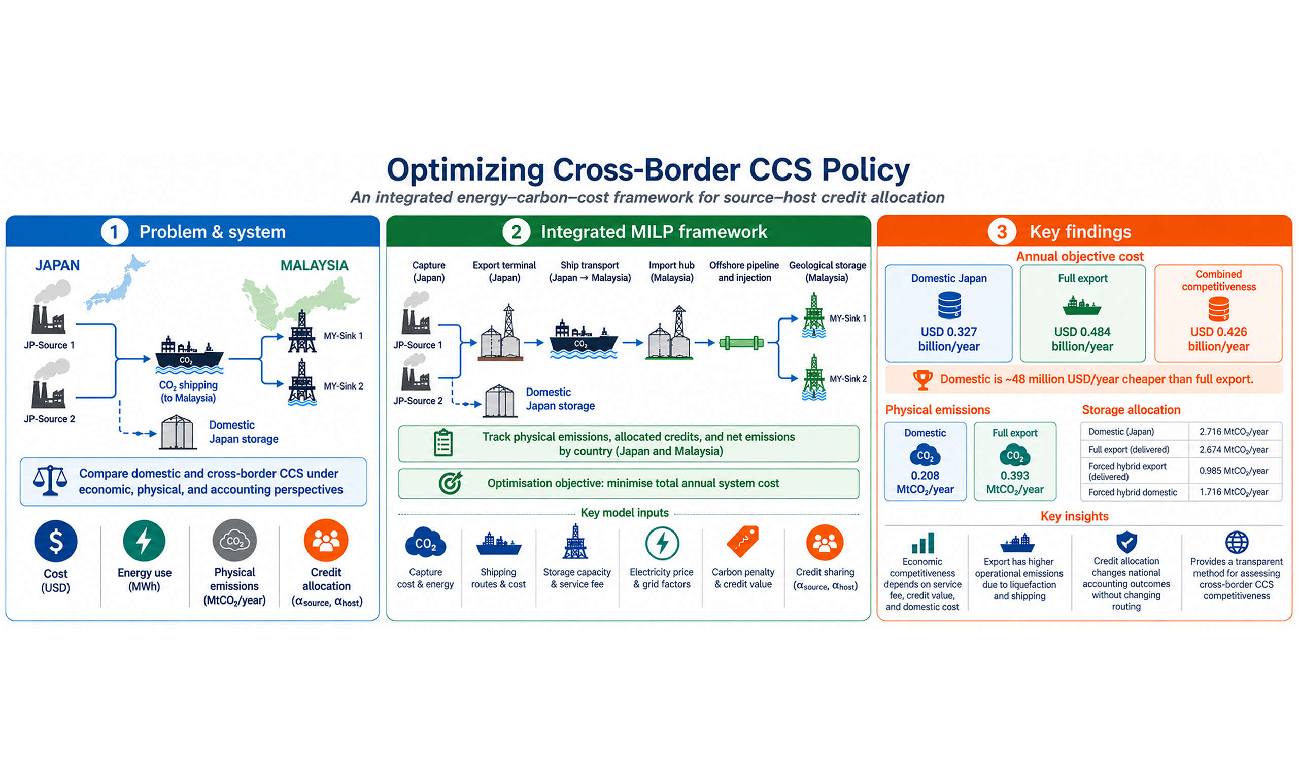
Cross-border carbon capture and storage (CCS) can support industrial decarbonisation where emissions and storage resources are unevenly distributed. Existing optimisation studies mainly minimise techno-economic cost and rarely integrate energy penalties, country-level emissions accounting, domestic-versus-export allocation, and source–host credit sharing. This study develops a mixed-integer linear programming framework that selects domestic or export storage, shipping routes, offshore pipelines, and sinks while tracking operational emissions, costs, and source–host credit allocation. An anonymised Japan–Malaysia case includes two Japanese sources, two Malaysian sinks, and a domestic screening pathway. Domestic Japanese storage costs USD 0.327 billion/year, compared with USD 0.484 billion/year for full export. Under the Combined Competitiveness scenario, a combination of a lower Malaysian service fee, equal source–host credit sharing, and an upper-end published domestic-storage cost selects full export to MY-Sink 1 at USD 0.426 billion/year, with the capability of storing 2.674 MtCO2/year after shipping loss. Credit ownership changes economic and national accounting outcomes without changing routing. Malaysian storage and injection, shipping, and credit values give the largest local sensitivity responses. In summary, the framework provides a transparent method for assessing cross-border CCS competitiveness, operational emissions, and sink selection.
Keywords
INTRODUCTION
Deep decarbonisation requires mitigation options for residual and process-related emissions from cement, steel, refining, chemicals, petrochemicals, and power generation. Carbon capture and storage (CCS) can address these hard-to-abate emissions through an integrated chain of capture, conditioning, transport, injection, monitoring, and geological storage. Deployment is increasing, but current and announced capacities remain below those required for net-zero pathways[1,2], which suggests the need to strengthen efficient full-chain planning.
CCS optimisation has traditionally focused on source–sink matching, transport-network design, pipeline sizing, storage allocation, and capacity expansion[3-5]. Several studies improved the representation of shipping, ports, offshore pipelines, and storage logistics[6-9]. These models establish a strong engineering basis for network design, but most emphasise techno-economic configuration. Energy-related emissions are often treated indirectly or assessed after optimisation, and the benefit of verified storage is rarely allocated explicitly between participating jurisdictions.
This limitation is important for cross-border CCS. Capture electricity, maritime transport, offshore pipeline transfer, and injection generate emissions in different countries, so stored CO2 and net mitigation are not equivalent. The source country may seek recognition for avoided industrial emissions, whereas the host country provides storage capacity, infrastructure, monitoring, and long-term stewardship. Existing environmental studies support full-chain assessment[10-12], while continuing advances in capture materials demonstrate the broader development of efficient CO2 separation technologies[13]. However, optimisation models seldom connect energy use, national emissions balances, route and sink decisions, and source–host benefit allocation within one formulation.
In this study, four related gaps are addressed: incomplete representation of full-chain energy penalties; limited country-level physical-emissions accounting; absence of an explicit rule for allocating the verified storage benefit without double counting; and limited comparison of optimised export pathways with a domestic-storage alternative. Addressing these gaps, an integrated energy–carbon–cost framework is required which links physical flows, infrastructure choices, operational emissions, policy values, and jurisdictional accounting. Therefore, this study develops a mixed-integer linear programming framework with four contributions. It integrates capture, shipping, offshore-pipeline, and injection energy with CO2 flows; formulates physical, credited, and net-emissions balances for source and host countries; introduces α-source and α-host shares for hypothetical source-claim, host-claim, and shared-credit cases; and compares domestic storage with cross-border export within a common scenario structure. The framework is demonstrated using an anonymised Japan–Malaysia system with two Japanese sources and two Malaysian offshore sinks.
METHODOLOGY
Generalised problem statement and system boundary
The optimisation problem is formulated as a general framework for cross-border CCS network design and operation. The proposed framework accommodates CCS systems involving multiple CO2 emission sources, domestic and foreign storage alternatives, transport routes, infrastructure options, jurisdictions, and policy scenarios. The case-specific source locations, storage sites, transport distances, costs, capacities, and policy parameters are introduced later in the case study section.
Given a set of CO2 emission sources i ∈ I, candidate storage sinks j ∈ J, transport routes r ∈ R, transport modes m ∈ M, countries or jurisdictions k ∈ K, operating periods t ∈ T, infrastructure options d ∈ D, and policy scenarios s ∈ S, the model determines the least-cost configuration and operation of the CCS chain. The storage set J may be divided into domestic storage alternatives JD and foreign or cross-border storage sinks JF. A general CCS superstructure is depicted in Figure 1.
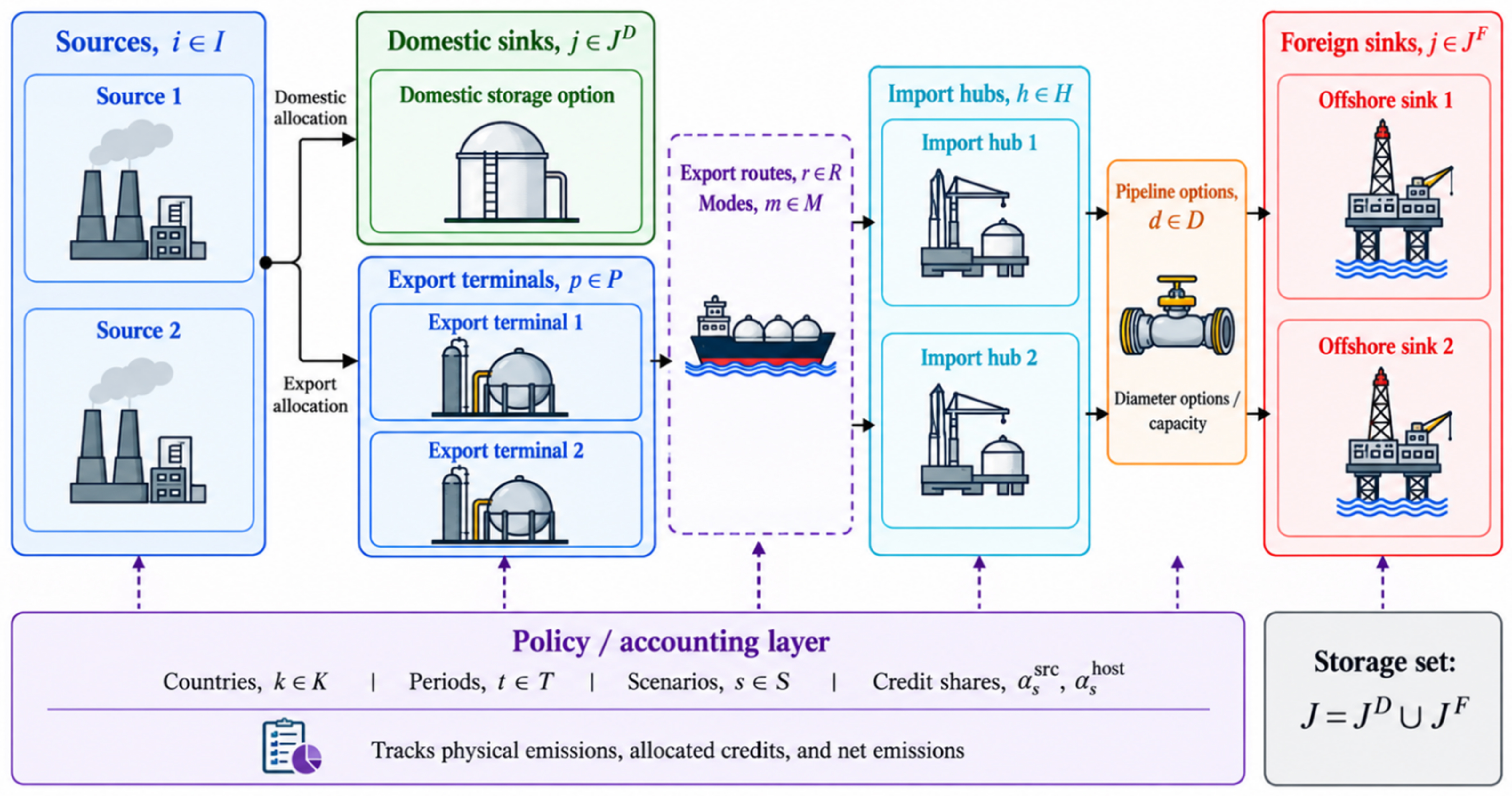
Figure 1. General CCS superstructure from source to storage. CCS: Carbon capture and storage.
Therefore, captured CO2 can be allocated either to domestic storage or to cross-border export routes. The cross-border pathway links source-country capture and export activities with host-country import, transport, injection, and geological storage activities. This structure allows the same optimisation framework to evaluate domestic-versus-export storage decisions, route and sink selection, infrastructure sizing, energy use, emissions accounting, and carbon-credit allocation.
The decision problem is to determine the amount of CO2 captured, uncaptured, transported, lost, injected, and stored; the routes, modes, sinks, and infrastructure options selected; the energy consumed by capture, conditioning, transport, and injection; and the country-level physical emissions, allocated credits, and net emissions. The objective is to minimise total annual system cost, including capture, transport, storage, energy, infrastructure, risk or access premiums, carbon penalties, and carbon-credit benefits, while satisfying mass-balance, capacity, loss, storage, energy, accounting, and policy constraints. Table 1 summarises the general sets and system elements used in the optimisation framework.
Generalised sets and system elements in the cross-border CCS optimisation framework
| Set/element | Symbol | Description |
| CO2 sources | i ∈ I | Emission sources where CO2 can be captured |
| Storage sinks | j ∈ J | Candidate geological storage alternatives |
| Domestic storage sinks | j ∈ JD | Storage alternatives located in the source country |
| Foreign storage sinks | j ∈ JF | Storage alternatives located in the host country |
| Transport routes | r ∈ R | Feasible source–hub–sink transport pathways |
| Transport modes | m ∈ M | Available CO2 transport modes |
| Export terminals | p ∈ PE | Loading or export-port systems |
| Import hubs | h ∈ H | Receiving hubs before storage transport |
| Countries/jurisdictions | k ∈ K | Source and host accounting jurisdictions |
| Time periods | t ∈ T | Operating or representative time intervals |
| Infrastructure options | d ∈ D | Discrete infrastructure choices |
| Scenarios | s ∈ S | Policy, market, and operational cases |
The generalised superstructure provides the basis for the mixed-integer linear programming (MILP) formulation. The model includes continuous variables for CO2 capture, export flow, domestic storage, hub flow, stored CO2, energy use, physical emissions, allocated credits, and net emissions. Binary variables indicate route and sink activation, while integer variables represent infrastructure-sizing decisions such as the number of offshore pipelines selected for each sink. The objective function and constraints are presented in the following subsections.
Objective function
The objective function minimises the total annual system cost. It includes CO2 capture, shipping and port services, annualised offshore-pipeline construction, host-country injection, storage and service charges, domestic transport and storage, pipeline and injection electricity, carbon penalties, and country-specific credit benefits.
The capture-cost coefficient is treated as an all-inclusive monetary proxy. Therefore, capture electricity is used to calculate physical emissions but is not charged separately in the objective function. Liquefaction and reconditioning electricity are treated in the same way because their monetary costs are already included in the corresponding port-service coefficients. This treatment prevents the same energy requirement from being counted twice.
where Z is the total annual objective cost; Ccap is the capture cost; Cship+port is the shipping and port-service cost; Cpipe,fix is the annualised offshore-pipeline construction cost; Cstore+service is the host-country injection, storage and service cost; Cdom is the domestic transport and storage cost in the source country; Celec is the separately charged offshore-pipeline and injection electricity cost; Cpen is the carbon-penalty cost; and Bcredit is the monetary benefit obtained from the allocated storage credit.
The carbon-credit benefit is calculated using country- and scenario-specific credit values:
where Bscredit is the total annual credit benefit under scenario s; H is the horizon-to-year scaling factor; K is the set of participating countries; T is the set of representative operating periods; Pk,scredit is the credit value applied by country k under scenario s; and Crk,t,s is the verified storage credit allocated to country k in period t under scenario s.
This formulation allows the same physical amount of stored CO2 to have different monetary values depending on the credit value and the share assigned to the source and host countries. Credit allocation affects economic and accounting outcomes but does not change the physical storage location.
The expanded annual objective function is:
where cicap is the capture-cost coefficient for source i; xi,t is CO2 captured from source i in period t; crship+port is the shipping and port-service cost for route r; fr,t is the gross CO2 flow on route r; cj,sstore+service is the injection, storage, and service-cost coefficient for foreign sink j under scenario s; zj,t is CO2 stored at sink j; ci,sdom is the domestic transport-and-storage cost for source i; di,tdom is CO2 assigned to domestic storage;
Variable operating costs are multiplied by H, whereas annualised pipeline-construction costs are added once outside the scaling term. Capture, liquefaction, and reconditioning electricity contribute to physical emissions but are not charged separately because their monetary costs are included in the corresponding capture and port-service coefficients.
Mass balance and physical constraints
The physical constraints conserve CO2 from its source to domestic or foreign storage. They also enforce capture limits, route capacities, transport losses, injection capacities, storage limits, import restrictions, and infrastructure-selection requirements.
The source balance divides gross emissions into captured and uncaptured CO2:
where xi,t is CO2 captured from source i in period t; ui,t is uncaptured CO2 released from source i; Ei,t is the gross CO2 emission from source i; I is the set of emission sources; and T is the set of operating periods.
The technical capture fraction limits the share of source emissions that can be captured:
where ηi is the maximum technically achievable capture fraction for source i; Ei,t is the gross source emission; and xi,t is the captured quantity.
The installed capture capacity provides a separate physical limit:
where
Captured CO2 can be allocated to domestic storage or cross-border export:
where Ri is the set of export routes connected to source i; fr,t is the CO2 exported through route r; and di,tdom is the CO2 assigned to domestic storage in the source country.
Export flow is permitted only when the corresponding route is activated:
where fr,t is the export flow on route r;
CO2 arriving at the host-country import hub is calculated after shipping losses:
where hj,t is the CO2 arriving at the import hub serving foreign sink j; Rj is the set of routes supplying sink j; λrship is the shipping-loss fraction for route r; and fr,t is the gross exported quantity.
The quantity stored at a foreign sink is calculated after offshore-pipeline losses:
where zj,t is the CO2 stored at foreign sink j; hj,t is the CO2 entering the offshore pipeline; and λjpipe is the offshore-pipeline operating-loss fraction.
The case study uses λjpipe = 0, meaning that all CO2 entering the offshore pipeline is assumed to reach the sink. This does not mean pipeline leakage is physically impossible. It means that no unsupported routine-loss value is imposed when project-specific operating-loss data are unavailable. The equation permits a verified non-zero value in future applications.
Hub flow cannot exceed the foreign-available injection capacity of the selected sink:
where
Annualised storage cannot exceed the available geological capacity:
where H is the horizon-to-year scaling factor; zj,t is stored CO2 in period t; and
The host-country import cap limits total cross-border delivery:
where
A minimum-export constraint is applied only in scenarios designed to require cross-border participation:
where Msmin is the minimum annual export requirement under scenario s; fr,t is the export flow; and H is the annual scaling factor. When Msmin = 0, the model is not required to export CO2.
Hub flow cannot exceed the installed offshore-pipeline capacity:
where
Pipeline construction is linked to sink activation:
where nj,d is the number of pipelines installed;
Energy modelling
Energy use is linked directly to CO2 flow at each operating stage. Capture and export-terminal liquefaction take place in the source country. Import-terminal reconditioning, offshore-pipeline transport, and injection take place in the host country. Domestic storage requires capture electricity together with the electricity used for domestic pipeline transport and injection.
Electricity use is first calculated in physical units and is then converted into emissions using the appropriate country grid-emission factor. Capture, liquefaction and reconditioning electricity are used for emissions accounting but are not charged separately because their costs are included in the corresponding service coefficients. Offshore-pipeline and injection electricity for the foreign-storage pathway are priced separately.
Capture electricity is proportional to the amount of CO2 captured:
where Ei,tcap is capture electricity use at source i; aicap is the capture-electricity coefficient; and xi,t is captured CO2.
Offshore-pipeline electricity depends on pipeline distance and transported CO2:
where Ej,tpipe is offshore-pipeline electricity use; ajpipe is the distance-based pipeline-energy coefficient; Djpipe is the offshore-pipeline distance to sink j; and hj,t is the CO2 entering the pipeline.
Injection electricity is proportional to the amount of CO2 stored:
where Ej,tinj is injection electricity use; ajinj is the injection-energy coefficient; and zj,t is the quantity injected and stored.
Shipping emissions are proportional to the gross quantity exported:
where SEt is direct shipping-related CO2 emissions in period t; arship is the shipping-emissions coefficient for route r; and fr,t is the gross CO2 flow transported through that route.
These energy requirements are included in the physical-emissions calculation but are not charged separately in the objective because their monetary contributions are included in the port-service coefficients.
Carbon accounting framework
The carbon-accounting framework separates physical operational emissions from allocated storage credits. This distinction is necessary because the country generating and capturing the CO2 may differ from the country providing transport, injection, and geological storage services.
The model first calculates the physical emissions assigned to each participating country:
where PEk,t is the total physical emission assigned to country k; UEk,t is uncaptured source emissions assigned to that country; EEk,t is grid-related emissions from CCS energy use occurring in that country; and SEk,t is direct shipping emissions assigned to that country under the modelled accounting boundary. Under the adopted boundary,
For the source country, physical emissions comprise uncaptured source emissions, grid emissions from capture and liquefaction, direct shipping emissions, and the energy-related emissions from domestic transport and injection when domestic storage is selected:
where
The domestic-storage emissions calculation includes the same quantified operating stages used for the export pathway: capture, pipeline transport, and injection. Monitoring is included in the monetary domestic-storage benchmark, but no separate monitoring-electricity value is added because the supporting source does not provide a defensible coefficient.
For the host country, physical emissions comprise electricity-related emissions from import-terminal reconditioning, offshore-pipeline transport and injection:
where
The anonymised foreign sinks use the same host-country grid-emission factor because they are assumed to operate within the same host-country electricity system. This value is a country-level case-study input rather than a site-specific measurement.
Net accounting emissions are calculated after the allocated storage credit is deducted from physical emissions:
where NEk,t,s is the net accounting-emission balance for country k under scenario s; PEk,t is the country’s physical operational emissions; and Crk,t,s is the verified storage credit allocated to that country.
A negative value of NEk,t,s indicates that the allocated accounting credit exceeds the physical emissions generated by the modelled CCS operations. It represents an accounting outcome and should not be interpreted as physically negative emissions.
Credit-sharing mechanism
The credit-allocation formulation is defined using an explicit source–sink mapping to avoid ambiguity in the allocation of verified stored CO2. Let Ai,j be a binary mapping parameter equal to 1 if captured CO2 from source i can be allocated to storage sink j, and 0 otherwise. The variable zi,j,t represents the amount of CO2 from source i that is finally stored in sink j during period t, after transport and storage losses have been accounted for. This source–sink-specific storage variable ensures that the verified stored CO2 is traced from its originating source to its final storage location.
The country-level credit allocated to country k in period t under scenario s is therefore expressed as:
where Crk,t,s is the CO2 storage credit allocated to country k in period t under scenario s, Ai,j is the source–sink mapping parameter, zi,j,t is the verified CO2 stored at sink j from source i, αssrc is the share of the storage credit allocated to the source country, and αshost is the share allocated to the host storage country. The binary indicator δi,ksrc equals 1 if source i is located in country k, and 0 otherwise. Similarly, δj,khost equals 1 if storage sink j is located in country k, and 0 otherwise.
To prevent double counting, the source and host credit shares are constrained as:
This formulation ensures that each unit of verified stored CO2 is allocated only once across the participating countries, subject to α_source + α_host = 1. A value of α_source = 1 assigns the full storage benefit to the source country, whereas α_host = 1 assigns it entirely to the host country. Intermediate values represent shared-benefit arrangements. The α parameters affect the allocation and monetary value of the verified storage benefit but do not change the physical CO2 flows or stored quantities. These cases are hypothetical policy scenarios used to test model behaviour and are not interpreted as established international carbon-accounting practices. In practice, the allocation rule would depend on bilateral agreements, domestic regulations, contractual terms, MRV requirements, infrastructure contributions, liability allocation, and agreed responsibilities for CO2 transport and long-term storage.
JAPAN–MALAYSIA CCS SYSTEM CASE STUDY
Case study system and network configuration
The case study represents an anonymised Japan–Malaysia cross-border CCS system with two Japanese CO2 source nodes, JP-Source 1 and JP-Source 2, and two Malaysian offshore storage sink nodes, MY-Sink 1 and MY-Sink 2. The pairing reflects a policy-relevant Asian source–host configuration: Japan represents a geographically compact industrial source country that may face a mismatch between future capture volumes and conveniently accessible domestic storage, whereas Malaysia represents a host country with emerging offshore storage ambitions. More broadly, the case illustrates how uneven distributions of industrial emissions and geological storage resources can motivate regional CO2 transport and storage cooperation[1,2]. JP-Source 1 represents a Japanese industrial CO2 source with access to marine export infrastructure. JP-Source 2 has different source and route characteristics, which allows the model to test whether multiple sources converge on the same Malaysian sink or select different sinks as costs, capacities, and transport conditions change. Two Malaysian offshore sinks, MY-Sink 1 and MY-Sink 2, differ in their transport requirements, injection capacities, and commercial conditions. The export network contains four feasible routes: JP-Source 1–MY-Sink 1, JP-Source 1–MY-Sink 2, JP-Source 2–MY-Sink 1, and JP-Source 2–MY-Sink 2. A domestic Japanese storage alternative, JP-Domestic Sink, is also included to compare cross-border export with a non-export pathway. Figure 2 shows the network and Table 2 summarises the modelling role of each node and route.
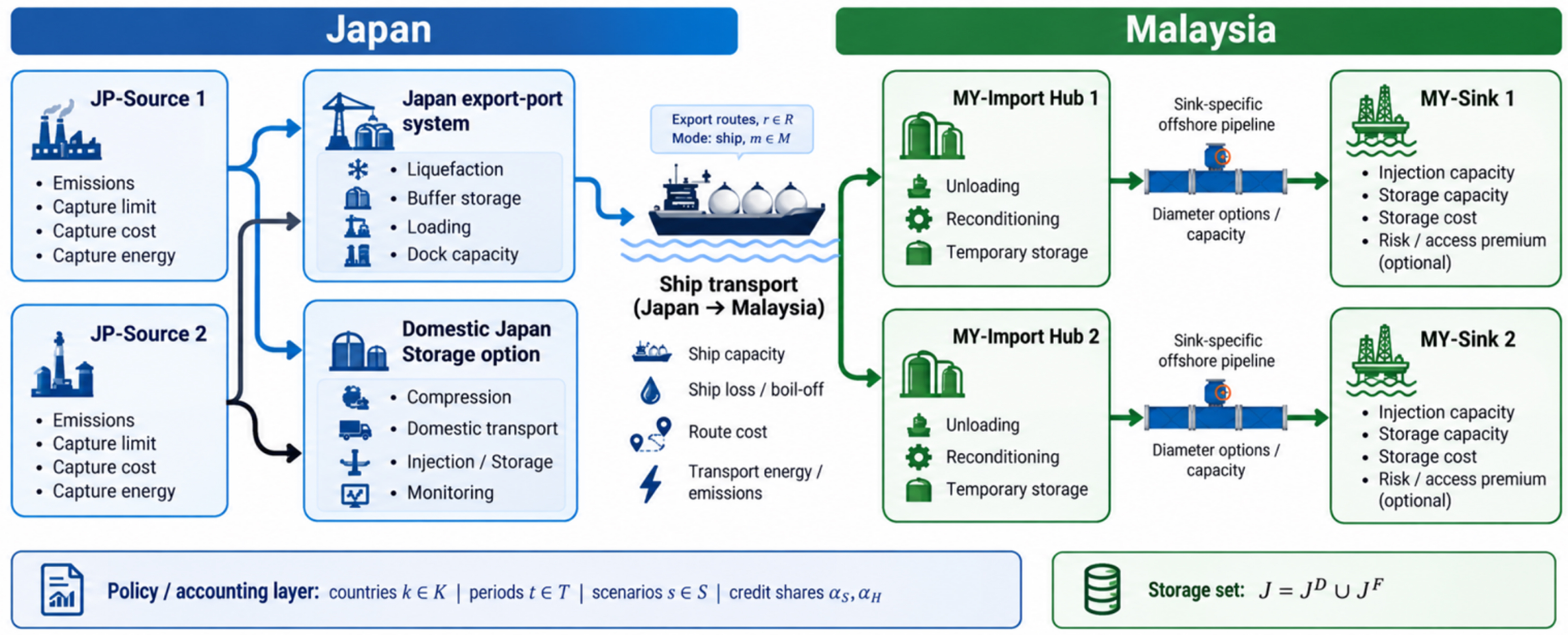
Figure 2. Cross-border CCS superstructure from Japan to Malaysia. CCS: Carbon capture and storage.
Node descriptions in the Japan–Malaysia case study
| Node/route | Description |
| JP-Source 1 | Japanese CO2 source node 1 |
| JP-Source 2 | Japanese CO2 source node 2 |
| MY-Sink 1 | Malaysian offshore storage sink 1 |
| MY-Sink 2 | Malaysian offshore storage sink 2 |
| MY-Import Hub 1 | Malaysian import hub 1 |
| MY-Import Hub 2 | Malaysian import hub 2 |
| Domestic Japan | Domestic Japan storage sink |
| JP-Source 1–MY-Sink 1 | Export route from JP-Source 1 to MY-Sink 1 |
| JP-Source 1–MY-Sink 2 | Export route from JP-Source 1 to MY-Sink 2 |
| JP-Source 2–MY-Sink 1 | Export route from JP-Source 2 to MY-Sink 1 |
| JP-Source 2–MY-Sink 2 | Export route from JP-Source 2 to MY-Sink 2 |
Case-study data and parameterisation
Inputs are grouped as fixed engineering and country data, literature-derived benchmarks, anonymised system assumptions, derived route values, and scenario settings. Table 3 identifies each group’s provenance, MILP role, and scenario dependence, distinguishing model inputs from contextual information.
Classification, provenance, modelling role, and scenario dependence of case-study inputs
| Parameter group | Parameters | Provenance | Model role |
| Source data | Emissions; capture limits | Literature-supported | Mass balance; capture limits |
| Capture | Cost; energy coefficient | Literature-supported | Cost; energy |
| Country | Electricity price; grid factor | Public data; proxy | Energy cost; emissions |
| Carbon policy | Penalty; credit value | Policy; market proxy | Cost; accounting |
| Domestic Japan | Compression; transport; storage; monitoring | Literature aggregate | Domestic pathway |
| Malaysian sinks | Capacity; injection; reservation | Anonymised assumptions | Storage constraints |
| Sink costs | Storage; injection | Literature-supported | Cost |
| Transport | Distance; cost; loss; emissions; pipeline | Assumed geometry; literature | Routing; cost; emissions |
| Commercial | Service fee; risk premium | Scenario assumptions | Cost; sink choice |
| Physical access | Import cap; minimum export | Scenario assumptions | Access constraints |
| Credit allocation | α source; α host | Hypothetical scenarios | Benefit allocation |
Source- and country-level parameters
The annual source emissions are anonymised case-study assumptions: JP-Source 1 emits 0.4 MtCO2/year, and JP-Source 2 emits 2.4 MtCO2/year. The maximum capture fraction is 0.97, following a high-capture precedent in Bennæs et al.[9]. The capture cost is set at USD100/tCO2 as an industrial proxy within published capture-cost evidence[14,15]. Capture electricity is set at 0.100 MWh/tCO2[16] and is used only for physical emissions. Japan’s electricity price is USD 86/MWh[17], while Malaysia’s electricity price remains USD 53.45/MWh[18]. Monetary values use USD 1 = MYR 4.06. Japan’s carbon penalty is a stated policy proxy of USD 26.85/tCO2[19]; Malaysia is assigned zero. Table 4 distinguishes literature-based values, public-data proxies, and explicit case-study assumptions.
Source- and country-level case-study parameters
| Model input | Value used | Unit | Basis | Reference |
| JP-Source 1 emissions | 0.4 | MtCO2/year | Anonymised assumption | Case-study design |
| JP-Source 2 emissions | 2.4 | MtCO2/year | Anonymised assumption | Case-study design |
| Maximum capture fraction | 0.97 | dimensionless | High-capture assumption | Bennæs et al.[9] |
| Capture cost | 100.00 | USD/tCO2 | Industrial literature-range proxy | Yu et al.[14]; Roussanaly et al.[15] |
| Capture electricity | 0.100 | MWh/tCO2 | Physical emissions only; cost embedded | Beiron et al.[16] |
| Japan electricity price | 86.00 | USD/MWh | Japan cost input | Isogai et al.[17] |
| Malaysia electricity price | 53.45 | USD/MWh | Common host electricity-price proxy | Sarawak Energy[18] |
| Japan grid-emission factor | 0.421 | tCO2/MWh | Official-data proxy | ANRE/METI[20] |
| Malaysia grid-emission factor | 0.199 | tCO2/MWh | Common host-grid proxy for both anonymised sinks | Energy Commission Malaysia[21] |
| Japan credit value | 18.62 | USD/tCO2 | Market proxy | JPX/TSE[22]; Bank Negara Malaysia[23] |
| Malaysia credit value | 12.32 | USD/tCO2 | Market proxy | Bursa Malaysia/BCX[24] |
| Japan carbon penalty | 26.85 | USD/tCO2 | Explicit policy proxy | Policy context[19] |
| Malaysia carbon penalty | 0 | USD/tCO2 | No verified numerical penalty applied | Case-study setting |
Storage-system parameters and domestic Japan benchmark
Domestic Japanese storage is represented as a screening pathway which compares export from capture at the source, transport through a 200 km onshore pipeline to injection, storage, and monitoring. The distance is an explicit case-study assumption, while the pipeline cost method, pipeline electricity, injection electricity, and storage-and-monitoring value are supported by published sources[17,25-30].
The domestic downstream cost is USD 18.33/tCO2. It comprises USD 4.11/tCO2 of annualised pipeline construction, USD 0.11/tCO2 of pipeline electricity, and the published Japanese storage-and-monitoring value of USD 14.10/tCO2[17]. Capture is added separately at USD 100/tCO2. Combined Competitiveness uses a higher downstream value of USD 64.23/tCO2: the same pipeline cost plus the USD 60/tCO2 upper-end onshore storage value reported in the storage-cost literature[28]. The higher value is used as a stress-test setting. Table 5 shows each component and calculation.
Literature-supported domestic Japan benchmark inputs
| Domestic component | Value used | Unit | Basis |
| Capture cost | 100.00 | USD/tCO2 | Industrial literature-range proxy[14,15] |
| Capture electricity | 0.100 | MWh/tCO2 | Physical emissions only[16] |
| Hypothetical pipeline distance | 200 | km | Case-study geometry; cost method[30] |
| Annualised pipeline construction | 4.11 | USD/tCO2 | 0.30-m pipeline; 7.5% capital charge[30] |
| Pipeline electricity | 0.11 | USD/tCO2 | 0.0013 MWh/tCO2 × USD86/MWh[17,25] |
| Storage and monitoring | 14.10 | USD/tCO2 | Japan benchmark[17] |
| Base downstream total | 18.33 | USD/tCO2 | Pipeline construction, electricity, storage and monitoring |
| Higher downstream total | 64.23 | USD/tCO2 | Combined competitiveness only; upper storage range[28] |
The energy boundary is kept consistent with the cost boundary. Capture electricity is not charged separately because it is already included in the all-inclusive capture cost. Domestic pipeline electricity is included in the downstream coefficient, and injection electricity is used to calculate physical emissions but is treated as embedded in the storage-and-monitoring value. No separate monitoring-electricity term is added because the cited Japanese benchmark does not report one; monitoring is retained within the monetary boundary described in the monitoring literature[31]. This avoids inventing an unsupported coefficient and prevents double counting.
The two Malaysian sinks are represented separately because of distinct geological inventories, annual injection rates, and route characteristics. MY-Sink 1 has 80 MtCO2 of storage and 3.7 MtCO2/year of injection capacity; MY-Sink 2 has 70 MtCO2 and 5.0 MtCO2/year. These capacities are anonymised case-study assumptions.
Table 6 distinguishes geological storage inventory from annual injection availability. Total storage capacity limits the amount stored over the project horizon, whereas injection capacity limits annual throughput. Keeping these constraints helps to separate and prevent a large geological inventory from being interpreted as unlimited yearly injection. The Malaysian storage-and-injection coefficient is represented as a composite USD 27.07/tCO2 proxy within published offshore-storage ranges[28,29].
Malaysian sink capacities, availability, costs, and pipeline distances
| Sink parameter | MY-Sink 1 | MY-Sink 2 | Unit | Basis |
| Total storage capacity | 80 | 70 | MtCO2 | Anonymised assumption |
| Gross injection capacity | 3.7 | 5.0 | MtCO2/year | Anonymised assumption |
| Domestic reservation | 0 | 0 | MtCO2/year | Disabled in all reported cases |
| Foreign-available capacity | 3.7 | 5.0 | MtCO2/year | Full stated injection capacity |
| Storage and injection | 27.07 | 27.07 | USD/tCO2 | Composite proxy within offshore range[28,29] |
| Offshore-pipeline distance | 190.6 | 205.8 | km | Hypothetical geometry |
| Routine pipeline loss | 0 | 0 | fraction | No verified project coefficient applied |
Transport and infrastructure parameters
Table 7 summarises the transport and infrastructure inputs. The anonymised route geometry produces shipping distances of 4,690.7-5,830.7 km and offshore-pipeline distances of 190.6 km to MY-Sink 1 and
Transport and infrastructure parameters
| Transport/infrastructure input | Value used | Unit | Basis/supporting source |
| Ship speed | 14 | Knots | Bennæs et al.[9] |
| Ship boil-off rate | 0.001 | Fraction per 12-hour period | Bennæs et al.[9] |
| Shipping-emissions coefficient | 0.013 | tCO2 emitted/tCO2 transported | Approximately 1.3%[9] |
| Liquefaction cost | 4.31 | USD/tCO2 | Roussanaly et al.[7]; Bennæs et al.[9] |
| Reconditioning cost | 1.56 | USD/tCO2 | Roussanaly et al.[7]; Bennæs et al.[9] |
| Port-handling cost per terminal | 0.20 | USD/tCO2 | Roussanaly et al.[7]; Bennæs et al.[9] |
| Liquefaction electricity | 0.134 | MWh/tCO2 | Isogai et al.[17] |
| Reconditioning electricity | 0.00271 | MWh/tCO2 | Isogai et al.[17] |
| Shipping cost coefficient | 0.00443 | USD/(tCO2·km) | Case-study assumption; dataset[32]; context[9,33-35] |
| Pipeline electricity | 0.0000065 | MWh/(tCO2·km) | Jaramillo et al.[25] |
| Injection electricity | 0.007 | MWh/tCO2 | Ottenbros et al.[26] |
| Capacity of 0.10-m pipeline | 35,100.83 | tCO2/month | Bennæs et al.[9] |
| Capacity of 0.15-m pipeline | 78,961.67 | tCO2/month | Bennæs et al.[9] |
| Capacity of 0.20-m pipeline | 140,342.50 | tCO2/month | Bennæs et al.[9] |
| Capacity of 0.30-m pipeline | 315,785.83 | tCO2/month | Bennæs et al.[9] |
| Pipeline-construction correlation | 0.533 + 0.019Q | Million EUR/km | Serpa et al.[30] |
| Construction-cost currency conversion | 5.00 | MYR/EUR | Fixed case-study financial assumption |
| Annual capital charge | 7.5 | %/year | Case-study financial assumption |
| Offshore-construction factor | 2.0 | Dimensionless | Serpa et al.[30] |
| Effective offshore-construction cost after factor | 1.333-1.490 | Million USD/km | Calculated from Serpa et al.[30] and stated currency assumptions |
| Maximum parallel pipelines per diameter | 5 | Pipelines | Non-binding numerical upper bound |
| Shipping-loss factor: JP1 → S1 | 0.0167 | Fraction | Calculated from Bennæs et al.[9] |
| Shipping-loss factor: JP1 → S2 | 0.0187 | Fraction | Calculated from Bennæs et al.[9] |
| Shipping-loss factor: JP2 → S1 | 0.0151 | Fraction | Calculated from Bennæs et al.[9] |
| Shipping-loss factor: JP2 → S2 | 0.0169 | Fraction | Calculated from Bennæs et al.[9] |
Shipping loss is calculated from distance, ship speed, the 12-hour boil-off period, and the published boil-off assumption[9]. The model values storage and credits using the amount that arrives after shipping loss. No routine offshore-pipeline loss is added in the numerical case. Port, line-haul shipping, pipeline construction, electricity, and storage services remain separate cost terms which make the route comparison auditable.
The shipping-cost coefficient of USD 0.00443/(tCO2·km) is treated as a case-study assumption informed by published CO2 shipping-cost studies[9,33-35], giving route-specific line-haul costs of USD 20.80-25.85/tCO2 for the assumed shipping distances. Liquefaction, reconditioning, and terminal-handling costs are based on the component cost rates reported by Bennæs et al.[9] which are € 3.50/tCO2 for liquefaction, € 1.27/tCO2 for reconditioning, and € 0.163/tCO2 for loading or unloading. Under the model conversion basis of RM5/€, these correspond to RM 17.50, RM 6.35, and RM 0.82/tCO2, respectively. Due to the handling occurring at both the export and import terminals, the total port-conditioning cost is RM 25.49/tCO2. At the reporting exchange rate of RM 4.06/USD, this equals USD 6.2783/tCO2. Therefore, the complete shipping-and-port range is USD 27.08-32.13/tCO2 after calculation.
Pipeline construction uses the published flow–cost correlation[30], MYR 5.00/EUR conversion, 7.5% annualisation, and a 2.0 offshore factor. The base cost of USD 0.666-0.745 million/km becomes USD 1.333-1.490 million/km offshore. Four diameter options (0.10-0.30 m) are used, with a non-binding limit of five parallel pipelines per diameter. Pipeline electricity is 0.0000065 MWh/(tCO2·km) scaled from
Export uses 0.134 MWh/tCO2 for liquefaction in Japan and 0.00271 MWh/tCO2 for reconditioning in Malaysia[17]. These coefficients affect emissions, while their electricity costs remain embedded in the port costs. Pipeline and injection electricity are priced separately. Both anonymised sinks use the same host-country electricity price and grid-emission factor.
Engineering assumptions
Assumptions include the 200-km domestic pipeline, anonymised source and sink capacities, shipping cost coefficient, currency conversion, annual capital charge, and numerical pipeline limit. Literature-based energy and emission coefficients are listed in Table 7. All reported cases set the MY-Sink 1 reservation, sink premiums, Malaysian carbon penalty, and routine offshore-pipeline loss to zero.
Flows, energy use, variable costs, and accounting quantities are calculated on a monthly-average basis. Annual source emissions and injection capacities are divided by 12 before entering monthly constraints, while monthly operating terms are multiplied by 12 for annual reporting. Annualised fixed infrastructure costs are added once. This consistent conversion prevents fixed costs from being repeated and keeps every flow and capacity on the same time basis. Seasonal vessel schedules, outages, and changing monthly injectivity are outside the deterministic model.
The principal case-study inputs are summarised in the main manuscript, while the complete numerical dataset, source–sink route matrix, scenario-specific parameter settings, and parameter-provenance classification are available in the Zenodo repository[32]. The all corresponding parameters are provided in the Supplementary Materials.
Scenario design
The scenario design is divided into four categories to represent the main decision dimensions in cross-border CCS, which include physical pathway selection, commercial and policy support, access constraints, and accounting allocation. This structure allows the analysis to examine how each dimension affects the economic competitiveness, CO2 allocation, and distribution of verified-storage benefits between the source and host countries.
Reference pathways represent the two basic CCS options considered in the model, which are exporting CO2 to Malaysia or storing it domestically in Japan. The commercial and policy-support scenarios then examine whether changes in economic conditions can improve the competitiveness of cross-border storage. The Low-Fee case reduces the Malaysian storage-service fee, while the Credit Support case introduces a storage-related credit benefit. Combined Competitiveness applies three favourable conditions together, which are a lower Malaysian storage-service fee, equal sharing of the storage credit between Japan and Malaysia, and higher domestic storage cost in Japan. Both domestic storage and export remain available, which allows the model to determine which pathway is preferred under these conditions.
The physical-access category examines whether an allocation requirement changes this decision. In the Forced Hybrid case, at least 1.0 MtCO2/year must be exported to Malaysia, while the remaining CO2 may still be stored in Japan. This represents a participation or access requirement.
The credit-allocation scenarios focus only on how the verified-storage benefit is shared between the two countries. The physical export system is kept unchanged, while the allocation parameters are varied. The Source Claim case assigns the full benefit to Japan (αsource = 1), Shared Credit divides it equally (0.5, 0.5), and Host Claim assigns the full benefit to Malaysia (αhost = 1). In all cases, αsource + αhost = 1 to ensure that the same storage benefit is counted only once. Credit Support and Combined Competitiveness use equal sharing between the two countries.
No storage credit is applied in the Reference, Low-Fee, or Forced Hybrid cases. When the credit mechanism is enabled, the benefit for each tonne stored is calculated from the shares assigned to Japan and Malaysia and their respective credit values. The credit changes the economic value of storage but does not change the physical location of the stored CO2. MY-Sink 1 reservation and sink risk premiums are set to zero in all reported scenarios. Table 8 summarises the inputs changed in each scenario; all other model inputs remain unchanged.
Scenario categories, scenario names, settings, and analytical purposes
| Scenario category | Scenario name | Pathway | Import cap (MtCO2/year) | Min. export (MtCO2/year) | MY fee (USD/tCO2) | Japan downstream cost (USD/tCO2) | Setting |
| Reference pathways | Base export | Export | 8.7 | 0 | 12.32 | NA | No credit; no reservation or premium |
| Reference pathways | Domestic Japan | Domestic | 0 | 0 | NA | 18.33 | 200 km screening pathway |
| Commercial and policy support | Low fee | Export | 8.7 | 0 | 6.16 | NA | Lower Malaysian service fee |
| Commercial and policy support | Credit support | Export | 8.7 | 0 | 12.32 | NA | Credits; αsource = αhost = 0.5 |
| Commercial and policy support | Combined competitiveness | Both | 8.7 | 0 | 6.16 | 64.23 | Low fee; shared credits; upper-end domestic cost |
| Physical-access constraints | Forced hybrid | Both | 8.7 | 1.0 | 12.32 | 18.33 | Minimum export requirement |
| Credit-allocation cases | Source claim | Export | 8.7 | 0 | 12.32 | NA | α source = 1; αhost = 0 |
| Credit-allocation cases | Shared 50:50 | Export | 8.7 | 0 | 12.32 | NA | α source = 0.5; αhost = 0.5 |
| Credit-allocation cases | Host claim | Export | 8.7 | 0 | 12.32 | NA | α source = 0; αhost = 1 |
RESULTS AND DISCUSSION
Overall scenario performance and pathway selection
This section examines how changes in economic support, physical-access conditions, and credit allocation affect the total system cost and selected CCS configuration. Table 9 presents the selected pathway, storage sink, CO2 flow, operational emissions, and annual objective cost according to the four scenario categories defined in Section “Scenario design”.
Overall outcomes by scenario
| Panel A. Reference pathways, commercial and policy support, and physical-access constraints | |||||||
| Scenario category | Scenario name | Objective cost (USD billion/year) | Export to MY (MtCO2/year) | Domestic storage (MtCO2/year) | Stored in MY (MtCO2/year) | Selected sink | Operational emissions (MtCO2/year) |
| Reference pathways | Base export | 0.484 | 2.716 | 0 | 2.674 | MY-Sink 1 (both sources) | 0.393 |
| Reference pathways | Domestic Japan | 0.327 | 0 | 2.716 | 0 | Not applicable | 0.208 |
| Commercial and policy support | Low-fee | 0.468 | 2.716 | 0 | 2.674 | MY-Sink 1 (both sources) | 0.393 |
| Commercial and policy support | Credit support | 0.443 | 2.716 | 0 | 2.674 | MY-Sink 1 (both sources) | 0.393 |
| Commercial and policy support | Combined competitiveness | 0.426 | 2.716 | 0 | 2.674 | MY-Sink 1 (both sources) | 0.393 |
| Physical-access constraints | Forced hybrid | 0.397 | 1.000 | 1.716 | 0.985 | MY-Sink 1 | 0.276 |
| Panel B. Credit-allocation cases | |||||||
| Scenario category | Allocation case | α source | α host | Credit benefit (USD million/year) | Objective cost (USD billion/year) | Physical pathway | Flow changed? |
| Credit-allocation cases | Source claim | 1.0 | 0.0 | 49.79 | 0.434 | Full export to MY-Sink 1 | No |
| Credit-allocation cases | Shared 50:50 | 0.5 | 0.5 | 41.36 | 0.443 | Full export to MY-Sink 1 | No |
| Credit-allocation cases | Host claim | 0.0 | 1.0 | 32.94 | 0.451 | Full export to MY-Sink 1 | No |
Under the reference assumptions, Base Export has an annual objective cost of USD 0.484 billion, compared with USD 0.327 billion for the Domestic Japan benchmark. Both pathways capture 2.716 MtCO2/year. However, the export pathway stores 2.674 MtCO2/year in Malaysia after shipping losses, whereas the domestic pathway stores the full captured amount in Japan.
Commercial and policy support reduces the cost disadvantage of cross-border storage. The Low-Fee, Credit Support, and Combined Competitiveness cases reduce the annual objective cost to USD 0.468 billion, USD 0.443 billion, and USD 0.426 billion, respectively. In the Combined Competitiveness case, the model selects full export to MY-Sink 1 instead of the upper-end domestic alternative available within that scenario. Nevertheless, its cost remains approximately USD 99 million/year above the base domestic screening benchmark. Therefore, the result demonstrates that export can become competitive under a coordinated set of favourable conditions, but it does not establish that export is universally cheaper than domestic storage.
All unconstrained export cases select MY-Sink 1 because it has the lower delivered transport cost. The Forced Hybrid case produces a different physical configuration because the minimum-export requirement prevents the model from selecting a fully domestic pathway. It exports 1.000 MtCO2/year, of which 0.985 MtCO2/year is stored in Malaysia after shipping losses, while the remaining 1.716 MtCO2/year is stored in Japan.
Credit allocation changes the distribution and monetary value of the verified storage benefit without changing the physical route or storage location. The Source Claim, Equal Sharing, and Host Claim cases provide annual credit benefits of USD49.79 million, USD41.36 million, and USD32.94 million, respectively. Their corresponding objective costs are USD0.434 billion, USD0.443 billion, and USD0.451 billion. All three cases retain full export to MY-Sink 1. The lower objective under Source Claim occurs because the modelled source-country credit value is higher than the host-country value, rather than because of a change in the physical CCS system.
Overall, the results show that pathway selection depends on the combined effect of commercial conditions, policy support, and physical constraints. Fee reductions and carbon credits improve export competitiveness, while access requirements can directly change the allocation between domestic and cross-border storage. Credit ownership mainly affects how the economic benefit is shared and does not, by itself, change the selected route. These comparisons should still be interpreted cautiously because domestic storage is represented by an aggregate screening benchmark, whereas the export network is modelled in greater physical detail. Therefore, the results support strategic comparison and identification of switching conditions, rather than a definitive project-level ranking of domestic and cross-border storage.
The emissions reported in Table 9 follow a matched operational boundary covering uncaptured CO2, electricity-related emissions from capture, conditioning, pipeline transport and injection, and direct shipping emissions.
Economic competitiveness and cost drivers
This section examines the cost difference between domestic and cross-border storage, identifies the main cost components, and compares the modelled values with published CCS cost ranges. Figure 3 shows an annual objective cost of USD 484.19 million for Base Export and USD 326.96 million for Domestic Screening, which gives a difference of USD 157.23 million/year. The Low-Fee and Credit Support cases reduce the export cost to USD467.72 million/year and USD442.83 million/year, respectively. Combined Competitiveness further reduces the objective to USD426.36 million/year and selects export over its upper-end domestic alternative of USD64.23/tCO2. However, the base domestic pathway, at USD18.33/tCO2, remains cheaper.
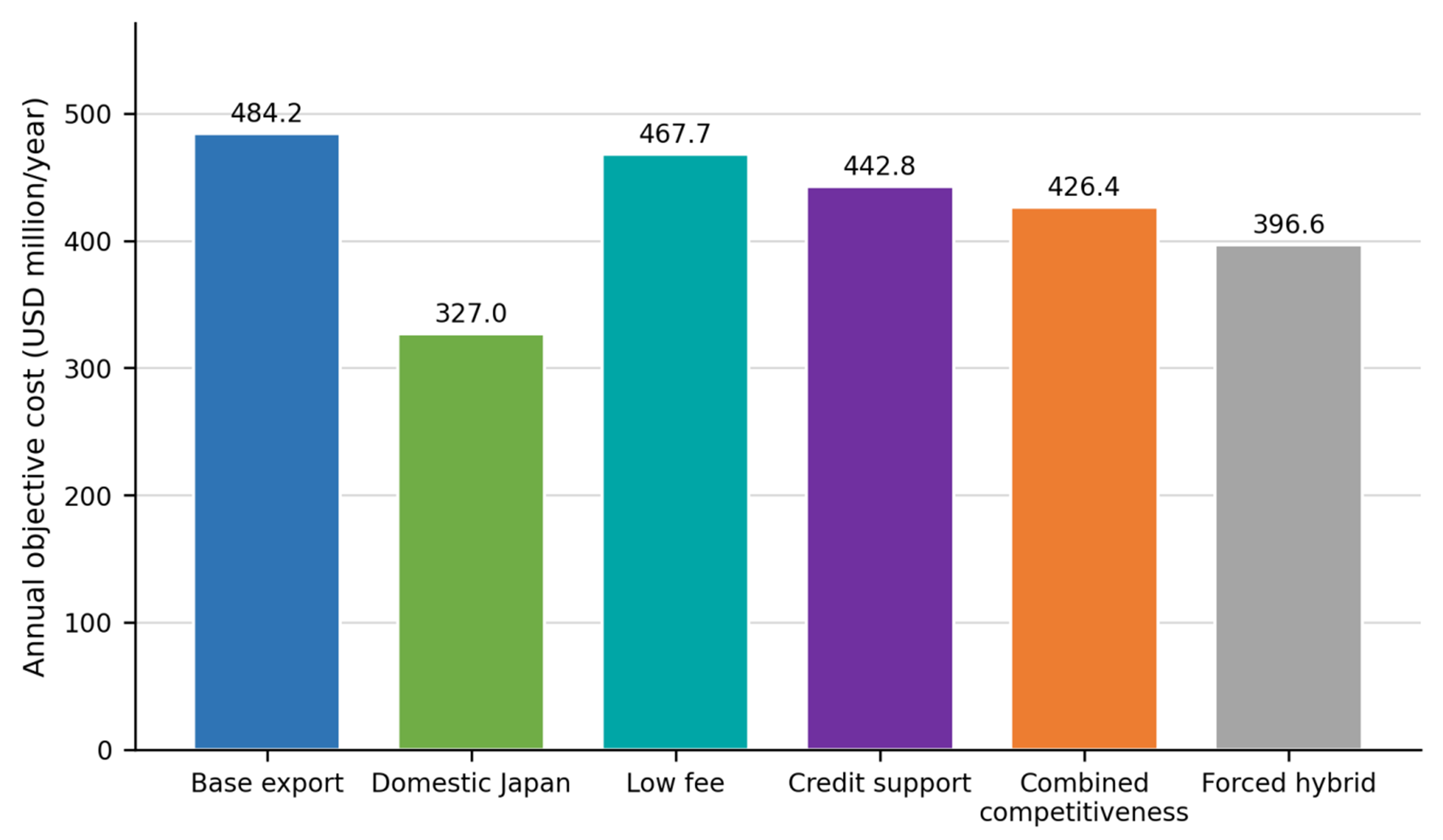
Figure 3. Annual objective cost across principal pathway scenarios.
Figure 4 compares the objective-cost components per tonne of CO2 captured. Capture contributes USD100/tCO2 in all three pathways. The net objectives are USD178.27/tCO2 for Base Export, USD120.38/tCO2 for Base Domestic Storage, and USD156.98/tCO2 for Combined Competitiveness. The lower service fee and shared carbon-credit benefit reduce the cost of the combined export case. Nevertheless, transport and host-country storage charges keep its objective above the base domestic benchmark.
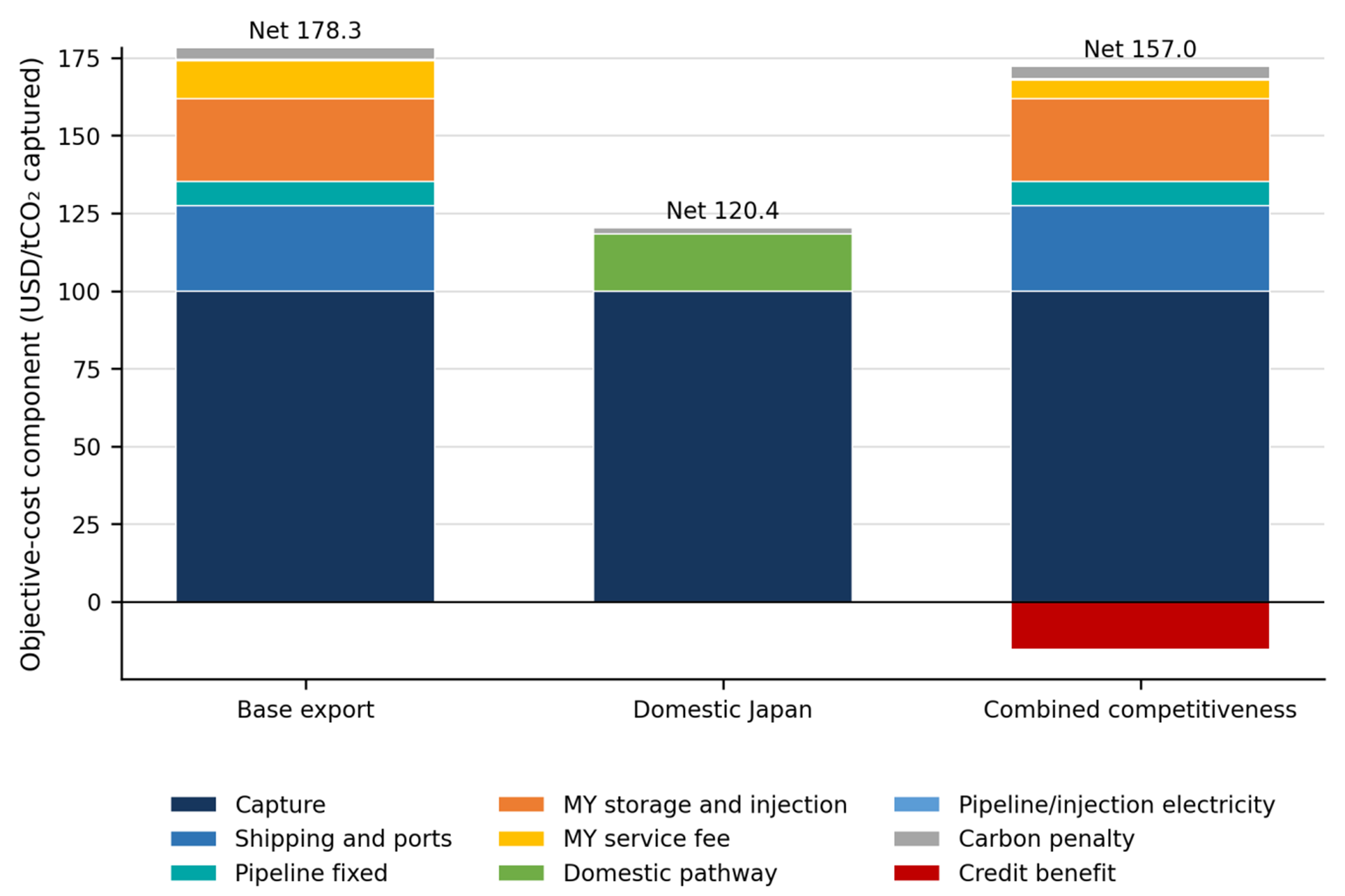
Figure 4. Cost-component decomposition of selected pathways on a common USD/tCO2-captured basis.
Recent optimisation studies cover source–sink networks[36], cluster and system abatement[37], multi-period supply chains[38-40], and industrial full-chain deployment[41,42]. Figure 5 provides a scale check using studies with sufficiently comparable ranges, together with earlier transport and full-chain estimates[9,15,17,28,43]. Cost scopes differ, so transport-only estimates cannot be ranked directly against objectives that include capture, conditioning, infrastructure, storage, penalties, and credits.
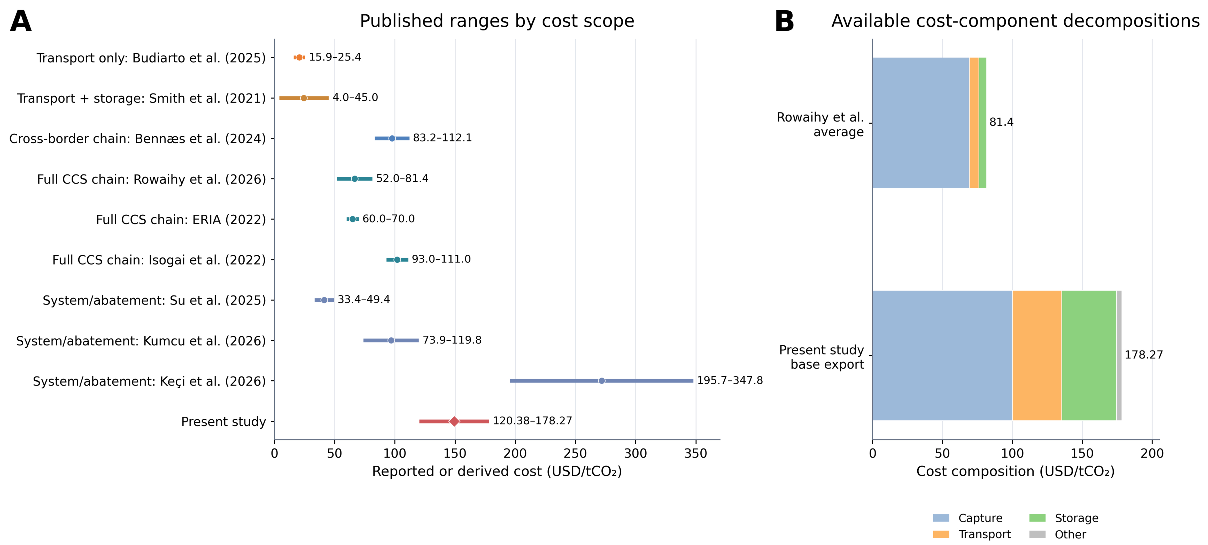
Figure 5. Published CCS/CCUS cost benchmarks by scope and available cost composition. (A) Published ranges by cost scope; (B) Available cost-component decompositions. CCS: Carbon capture and storage; CCUS: Carbon capture, utilisation and storage.
Overall, the results indicate that commercial and policy support can substantially reduce the cost of cross-border CCS, but it does not automatically make export cheaper than the lowest domestic benchmark. The Combined Competitiveness result is best interpreted as evidence of conditional competitiveness in which export becomes the preferred decision only when it is compared with the upper-end domestic alternative under the same scenario. The published ranges support the order of magnitude of the modelled costs, but these do not validate an exact project cost because the estimates depend on source type, transport distance, system capacity, financing assumptions, energy boundaries, and price year. Across the three pathways presented in Figure 4, capture remains the largest single positive cost component.
Network configuration, route and sink selection
Transport and storage characteristics influence route and sink selection. These include shipping distance, line-haul cost, shipping loss, offshore-pipeline distance, and injection capacity. In the Base Export case, both sources deliver CO2 to MY-Sink 1. Of the 2.716 MtCO2/year exported, 2.674 MtCO2/year is stored after a shipping loss of 1.53%. Compared with MY-Sink 2, the route to MY-Sink 1 is 638.3 km shorter and USD2.83/tCO2 cheaper for JP-Source 1. For JP-Source 2, it is 561.2 km shorter and USD2.49/tCO2 cheaper. The offshore pipeline serving MY-Sink 1 is also 15.2 km shorter. MY-Sink 1 receives 2.674 MtCO2/year, which remains below its injection capacity of 3.7 MtCO2/year. MY-Sink 2 provides a higher injection capacity of 5.0 MtCO2/year but is not selected because its additional capacity is unnecessary at the modelled flow and does not offset its higher transport cost. Figure 6 compares the route and sink attributes.
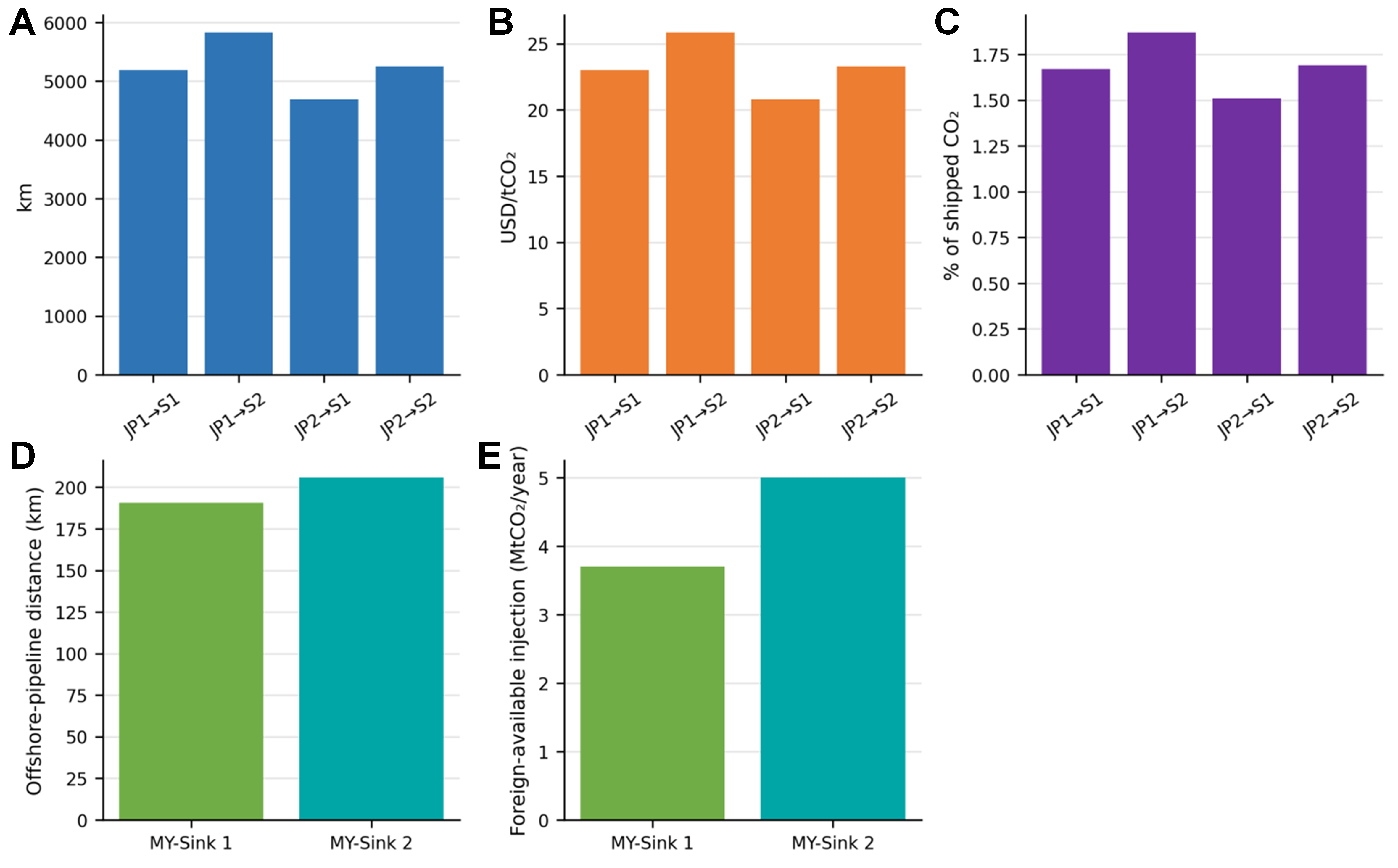
Figure 6. Route and sink performance for the two Japanese sources and Malaysian sinks. (A) Shipping distance; (B) Shipping cost; (C) Shipping-loss factor; (D) Offshore-pipeline distance; (E) Foreign-available injection capacity.
Overall, the result shows that lower delivered transport cost determines sink selection when both sinks have sufficient capacity and share the same storage assumptions. However, MY-Sink 2 may become preferable at higher CO2 flows, under tighter capacity conditions, or if its relative transport and storage costs decrease. Therefore, the selection of MY-Sink 1 should be interpreted as a result of the current case-study configuration.
Source–host credit allocation and accounting outcomes
This section explores how alternative credit-sharing arrangements affect the economic benefit and country-level accounting outcomes without changing the physical CCS system. All three α cases physically store 2.674 MtCO2/year in Malaysia at MY-Sink 1. The Source Claim, Equal Sharing, and Host Claim cases provide annual credit benefits of USD49.79 million, USD41.36 million, and USD32.94 million, respectively. Their corresponding annual objective costs are USD0.434 billion, USD0.443 billion, and USD0.451 billion. The difference arises because Japan has a higher modelled carbon-credit value than Malaysia. Therefore, the allocation of a larger share to Japan produces a greater economic benefit and a lower system objective.
Figure 7 separates physical emissions, allocated storage credit, and the resulting net accounting balance. Under Source Claim, the net balances for Japan and Malaysia are -2.287 and +0.006 MtCO2/year, respectively. Under Equal Sharing, the corresponding balances are -0.950 and -1.331 MtCO2/year. Under Host Claim, the net balances become +0.387 and -2.669 MtCO2/year. In every case, the CO2 remains physically stored in Malaysia, and only the ownership and monetary value of the accounting benefit change.
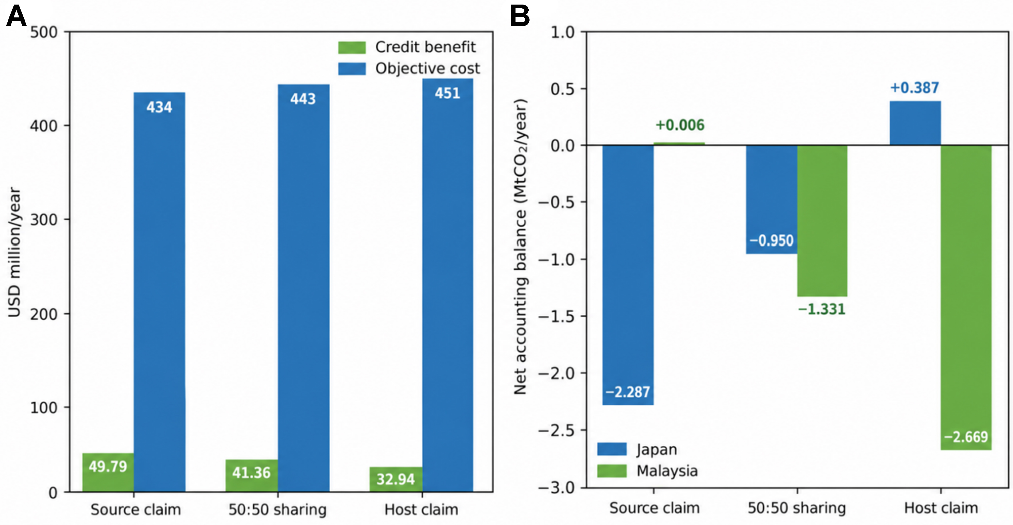
Figure 7. Economic and country-level accounting effects of source–host credit allocation (A) Economic effect; (B) Country-level accounting effect. Note: Accounting balances are calculated from unrounded model outputs and displayed values may not sum exactly because of rounding.
Overall, the results show that credit allocation can materially affect the distribution of economic and accounting benefits even when the physical route, storage sink, and stored quantity remain unchanged. The lowest objective under Source Claim reflects Japan’s higher assumed credit value, not a more efficient physical configuration.
Physical CO2 allocation and quantified emissions
A matched operational boundary is applied to compare the emissions generated by domestic, export, and hybrid CCS pathways. The resulting operational emissions are 0.208 MtCO2/year for Domestic Storage, 0.393 MtCO2/year for Base Export, and 0.276 MtCO2/year for Forced Hybrid. Base Export produces the highest operational emissions, mainly because it requires liquefaction electricity and long-distance shipping. Infrastructure-construction emissions and other full life-cycle effects are excluded from this comparison.
The Domestic Japan pathway stores the full captured quantity of 2.716 MtCO2/year. Base Export sends 2.716 MtCO2/year to Malaysia and stores 2.674 MtCO2/year after shipping losses. Forced Hybrid exports 1.000 MtCO2/year, of which 0.985 MtCO2/year is stored in Malaysia, while the remaining 1.716 MtCO2/year is stored in Japan. Figure 8 distinguishes the amount allocated to each pathway, the quantity reaching storage, and the associated operational emissions.
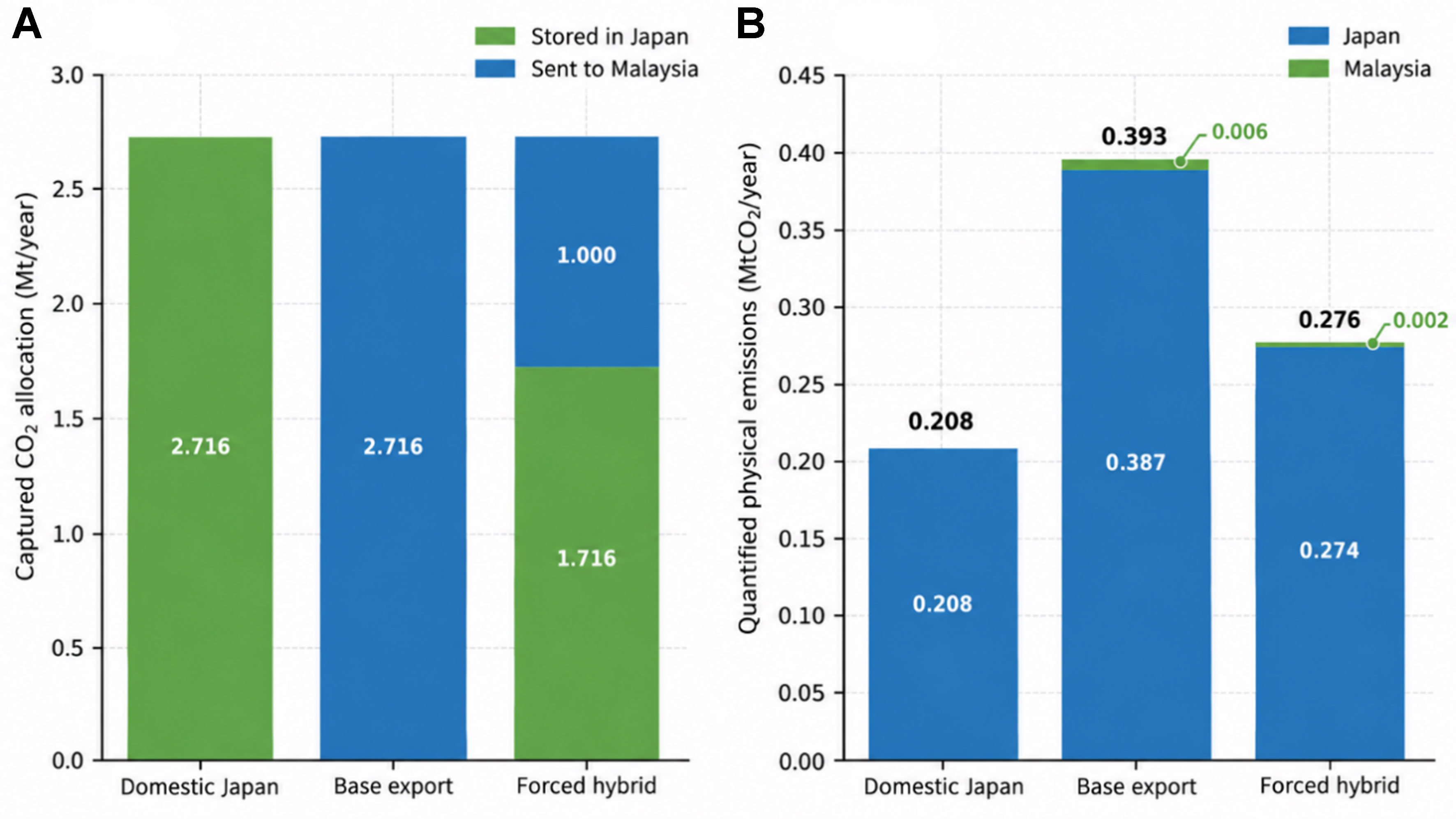
Figure 8. Physical CO2 allocation and matched-boundary operational emissions. (A) Domestic and export allocation; (B) Quantified operational emissions by country.
Overall, cross-border export achieves substantial CO2 storage but produces higher operational emissions and slightly lower delivered storage because of additional conditioning, shipping, and transport losses. Forced Hybrid lies between the fully domestic and fully exported pathways because it uses both systems. These results show the operational trade-off between accessing foreign storage and the additional energy and emissions required for cross-border transport.
Sensitivity analysis
The sensitivity analysis evaluates both cost responsiveness and decision stability around the Combined Competitiveness case. Figure 9 illustrates one-at-a-time (OAT) objective-cost responses. The reference applies a USD 6.16/tCO2 service fee, equal source–host credit shares, and a domestic downstream cost of USD 64.23/tCO2, while the domestic reservation and sink-specific premiums are set to zero.
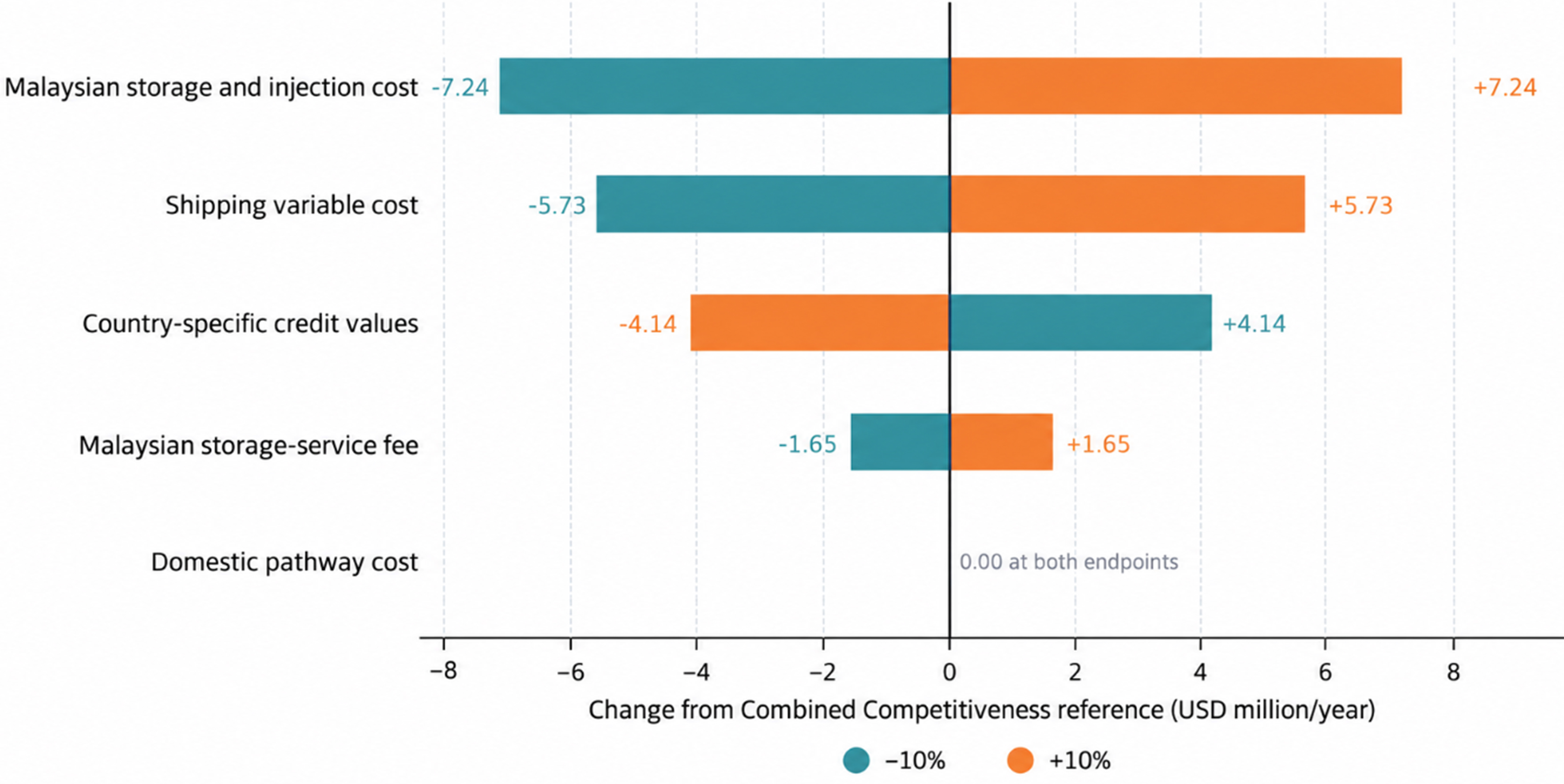
Figure 9. Combined competitiveness ±10% OAT objective-cost response. Each bar connects the -10% and +10% endpoints relative to the reference objective. OAT: One-at-a-time.
Five inputs are varied separately by ±10%: shipping cost, domestic pathway cost, country-specific credit values, service fee, and Malaysian storage-and-injection cost. In the credit test, the Japanese and Malaysian credit values change together by the same percentage. Each endpoint represents a separate MILP optimisation in which only one input changes, while all other inputs and scenario settings remain fixed.
The reference solution selects full export of 2.716 MtCO2/year to MY-Sink 1, with an annual objective cost of USD 426.358 million. Malaysian storage-and-injection cost produces the largest endpoint range at USD 14.478 million/year. This is followed by shipping cost at USD 11.469 million/year, credit values at USD 8.273 million/year, and the service fee at USD 3.294 million/year. Higher credit values reduce the objective because the credit is treated as an economic benefit. Domestic pathway cost has no local effect because the model retains full export at both endpoints.
None of the ±10% changes alter the selected pathway or sink; every optimisation continues to select full export to MY-Sink 1. This indicates that the Combined Competitiveness decision is locally stable within the tested ranges. However, the result does not show that the decision would remain unchanged under larger variations or simultaneous changes in several inputs. The zero response to domestic cost also does not mean that domestic cost is generally unimportant, as it remains inactive within this limited range.
Overall, the OAT analysis identifies the inputs that have the strongest local effects on the optimised cost and tests whether moderate individual changes alter the infrastructure decision. As a local analysis within a deterministic MILP, it does not account for probability distributions, correlations between uncertain inputs, or combined uncertainty. Wider-range, multi-parameter, or probabilistic analyses would be required to identify switching thresholds and assess broader decision risk.
CONCLUSION
This study develops an integrated MILP framework that links CCS pathway, route and sink selection with cost, operational emissions, and source–host credit allocation. Under the reference assumptions, base domestic storage costs USD 0.327 billion/year, compared with USD 0.484 billion/year for base export. The Combined Competitiveness case selects full export to MY-Sink 1 at USD 0.426 billion/year when compared with the upper-end domestic alternative, although it remains more expensive than the base domestic screening benchmark. Malaysian storage and injection costs, shipping costs, and carbon-credit values have the largest local effects on the objective, while the selected export pathway remains stable within the tested ±10% ranges. Credit allocation changes the distribution of economic and national accounting benefits without changing the physical route or storage location. Future work should apply project-specific data, model domestic and export networks at equal resolution, examine joint uncertainty and switching thresholds, and develop monitoring-linked rules for sharing verified storage benefits.
DECLARATIONS
Authors’ contributions
Conceptualization, investigation, data curation, formal analysis, writing - original draft: Ting, J. Z. Z.; Lim, J. S.
Methodology, validation, supervision, writing - review and editing: Ting, J. Z. Z.; Lim, J. S.
Writing - review and editing: Wan Alwi, S. R.; Abdul Manan, Z.; Wang, B.; Gai, L.
Availability of data and materials
The supporting dataset and model files are available in the Zenodo repository[32].
AI and AI-assisted tools statement
During the preparation of this manuscript, OpenAI ChatGPT (GPT-5.6, released 2026-07-09) was used to assist with language editing, produce the graphical abstract, and refine Figures 1 and 2. The AI tool did not influence the study design, data collection, mathematical formulation, model implementation, numerical analysis, interpretation of results, or the scientific conclusions of the work. All AI-assisted content was reviewed, verified, and revised by the authors, who take full responsibility for the final manuscript.
Financial support and sponsorship
None.
Conflicts of interest
All authors declared that there are no conflicts of interest.
Ethical approval and consent to participate
Not applicable.
Consent for publication
Not applicable.
Copyright
© The Author(s) 2026.
Supplementary Materials
REFERENCES
1. International Energy Agency. Carbon capture, utilisation and storage. https://www.iea.org/energy-system/renewables-and-low-emissions/carbon-capture-utilisation-and-storage. (accessed 2026-10-20).
2. Global CCS Institute. Global status of CCS 2024: collaborating for a net-zero future. https://www.globalccsinstitute.com/wp-content/uploads/2024/10/Global-Status-Report-6-November.pdf. (accessed 2026-10-20).
3. Middleton, R. S.; Bielicki, J. M. A scalable infrastructure model for carbon capture and storage: SimCCS. Energy. Policy. 2009, 37, 1052-60.
4. d’Amore, F.; Bezzo, F. Economic optimisation of European supply chains for CO2 capture, transport and sequestration. Int. J. Greenh. Gas. Control. 2017, 65, 99-116.
5. Zhang, S.; Liu, L.; Zhang, L.; Zhuang, Y.; Du, J. An optimization model for carbon capture utilization and storage supply chain: a case study in Northeastern China. Appl. Energy. 2018, 231, 194-206.
6. Roussanaly, S.; Bureau-Cauchois, G.; Husebye, J. Costs benchmark of CO2 transport technologies for a group of various size industries. Int. J. Greenh. Gas. Control. 2013, 12, 341-50.
7. Roussanaly, S.; Brunsvold, A. L.; Hognes, E. S. Benchmarking of CO2 transport technologies: Part II - Offshore pipeline and shipping to an offshore site. Int. J. Greenh. Gas. Control. 2014, 28, 283-99.
8. Kjärstad, J.; Skagestad, R.; Eldrup, N. H.; Johnsson, F. Ship transport - a low cost and low risk CO2 transport option in the Nordic countries. Int. J. Greenh. Gas. Control. 2016, 54, 168-84.
9. Bennæs, A.; Skogset, M.; Svorkdal, T.; et al. Modeling a supply chain for carbon capture and offshore storage - a German–Norwegian case study. Int. J. Greenh. Gas. Control. 2024, 132, 104028.
10. Boot-Handford, M. E.; Abanades, J. C.; Anthony, E. J.; et al. Carbon capture and storage update. Energy. Environ. Sci. 2014, 7, 130-89.
11. Bui, M.; Adjiman, C. S.; Bardow, A.; et al. Carbon capture and storage (CCS): the way forward. Energy. Environ. Sci. 2018, 11, 1062-176.
12. Becattini, V.; Gabrielli, P.; Antonini, C.; et al. Carbon dioxide capture, transport and storage supply chains: optimal economic and environmental performance of infrastructure rollout. Int. J. Greenh. Gas. Control. 2022, 117, 103635.
13. Shi, W.; Guo, Y.; Lu, Q.; et al. Dynamic tailoring of the gradient porosity of biomass-derived porous carbons for highly effective CO2 capture. Green. Chem. 2025, 27, 11416-28.
14. Yao, Y.; Marano, J.; Morrow, W. R.; Masanet, E. Quantifying carbon capture potential and cost of carbon capture technology application in the U.S. refining industry. Int. J. Greenh. Gas. Control. 2018, 74, 87-98.
15. Roussanaly, S.; Berghout, N.; Fout, T.; et al. Towards improved cost evaluation of carbon capture and storage from industry. Int. J. Greenh. Gas. Control. 2021, 106, 103263.
16. Beiron, J.; Normann, F.; Johnsson, F. A techno-economic assessment of CO2 capture in biomass and waste-fired combined heat and power plants - a Swedish case study. Int. J. Greenh. Gas. Control. 2022, 118, 103684.
17. Isogai, H.; Myers, C. A.; Nakagaki, T. Cost estimation of CCS integration into thermal power plants in Japan. Mech. Eng. J. 2022, 9, 22-00028.
18. Sarawak Energy Berhad. Tariff information. https://www.sarawakenergy.com/assets/pdf/tariff-info.pdf. (accessed 2026-10-20).
19. Ministry of Economy, Trade and Industry. Opinion on the FY2026 reference upper transaction price and adjustment benchmark transaction price (in Japanese). https://www.meti.go.jp/shingikai/sankoshin/sangyo_gijutsu/emissions_trading/pdf/20251219_2.pdf. (accessed 2026-10-20).
20. Agency for Natural Resources and Energy, Ministry of Economy, Trade and Industry. Electricity emission factors applied to the Green Energy CO2 Reduction Equivalent Certification System: FY2021 calculation results (in Japanese). https://www.enecho.meti.go.jp/category/saving_and_new/green_energy/newenergy/geco2_iinnkai/32doc2.pdf. (accessed 2026-10-20).
21. Energy Commission Malaysia. Grid emission factor (GEF) in Malaysia, 2022-2024. https://www.climatiq.io/data/source/energy-commission-of-malaysia. (accessed 2026-10-20).
22. Japan Exchange Group. The carbon trading marketplace in Japan. 2024. https://www.asean.or.jp/main-site/wp-content/uploads/2024/05/5-JPX-Carbon-Credit-Market_20240326.pdf. (accessed 2026-10-20).
23. Bank Negara Malaysia. Exchange rates. https://www.bnm.gov.my/latest-rates. (accessed 2026-10-20).
24. Bursa Malaysia. Bursa Carbon Exchange auctions first Malaysian nature-based carbon credits. 2024. https://www.skrine.com/insights/alerts/july-2024/bursa-carbon-exchange-auctions-first-malaysian-nat. (accessed 2026-10-20).
25. Jaramillo, P.; Griffin, W. M.; McCoy, S. T. Life cycle inventory of CO2 in an enhanced oil recovery system. Environ. Sci. Technol. 2009, 43, 8027-32.
26. Ottenbros, A. B.; van Zelm, R.; Simons, J.; et al. Prospective environmental burdens and benefits of fast-swing direct air carbon capture and storage. Sci. Rep. 2024, 14, 16549.
27. McCollum, D. L.; Ogden, J. M. Techno-economic models for carbon dioxide compression, transport, and storage and correlations for estimating carbon dioxide density and viscosity. Research Report UCD-ITS-RR-06-14. 2006. https://www.researchgate.net/publication/46440087_Techno-Economic_Models_for_Carbon_Dioxide_Compression_Transport_and_Storage_Correlations_for_Estimating_Carbon_Dioxide_Density_and_Viscosity. (accessed 2026-10-20).
28. Hatta, A.; Consoli, C.; Seyyedi, M. Cost of CO2 storage. Melbourne: Global CCS Institute; 2025. https://www.globalccsinstitute.com/wp-content/uploads/2025/12/Cost-of-CO2-Storage-1225.pdf. (accessed 2026-10-20).
29. Hendriks, C.; Graus, W.; van Bergen, F. Global carbon dioxide storage potential and costs. Utrecht: Ecofys; 2004. https://www.researchgate.net/publication/260095614_Global_Carbon_Dioxide_Storage_Potential_and_Costs. (accessed 2026-10-20).
30. Correia Serpa dos Santos, J.; Morbee, J.; Tzimas, E. Technical and economic characteristics of a CO2 transmission pipeline infrastructure. EUR 24731 EN. Luxembourg: Publications Office of the European Union; 2011.
31. IEAGHG. Monitoring and modelling of CO2 storage: the potential for improving the cost-benefit ratio of reducing risk. 2020. https://ieaghg.org/publications/monitoring-and-modelling-of-co2-storage/. (accessed 2026-10-20).
32. Ting, J. Z. Z.; Lim, J. S.; Wan, Alwi. S. R.; Abdul, Manan. Z.; Wang, B.; Gai, L. Optimizing cross-border CCS policy: an integrated energy–carbon–cost framework for source–host credit allocation. Zenodo 2026.
33. Decarre, S.; Berthiaud, J.; Butin, N.; Guillaume-Combecave, J. CO2 maritime transportation. Int. J. Greenh. Gas. Control. 2010, 4, 857-64.
34. Knoope, M.; Ramírez, A.; Faaij, A. A state-of-the-art review of techno-economic models predicting the costs of CO2 pipeline transport. Int. J. Greenh. Gas. Control. 2013, 16, 241-70.
35. Mccoy, S.; Rubin, E. An engineering-economic model of pipeline transport of CO2 with application to carbon capture and storage. Int. J. Greenh. Gas. Control. 2008, 2, 219-29.
36. Gu, C.; Zhu, C.; Gong, X.; et al. A novel source–sink matching optimization model for carbon capture and storage. Geol. J. 2025, 60, 1840-51.
37. Su, X. N.; Qiu, J. X.; Luan, L. M.; Mei, Y. D. Source-sink matching and cluster layout of carbon capture, utilization and storage in China towards carbon neutrality. Clim. Change. Res. 2025, 21, 373-86.
38. Budiarto, O.; Purwanto, W. W.; Halimatussadiah, A.; Maharsi, D. A. Multi-period superstructure optimization for CCS source-sink matching in South Sumatra industrial clusters. Carb. Neutrality. 2025, 4, 135.
39. Leonzio, G.; Foscolo, P. U.; Zondervan, E. Sustainable utilization and storage of carbon dioxide: analysis and design of an innovative supply chain. Comput. Chem. Eng. 2019, 131, 106569.
40. Kumcu, S.; Özyörük, B.; Bezzo, F.; d’Amore, F. Optimization of carbon capture, utilization, and storage supply chains for the hard-to-abate industry in Türkiye. Int. J. Greenh. Gas. Control. 2026, 150, 104568.
41. Rowaihy, F.; Hamieh, A.; Odeh, N.; et al. Decarbonizing Saudi Arabia’s energy and industrial sectors: an integrated techno-economic assessment of CCS. Energy. Convers. Manag. X. 2026, 29, 101536.
42. Keçi, H.; Alcani, M.; Dorri, A. Assessing the potential of carbon capture, utilization, and storage for industrial decarbonization. Int. J. Innov. Technol. Interdiscip. Sci. 2026, 9, 1371-88.
Cite This Article
 Open Access
How to Cite
Ting, J. Z. Z.; Lim, J. S.; Wan Alwi, S. R.; Abdul Manan, Z.; Wang, B.; Gai, L. Optimizing cross-border CCS policy: an integrated energy–carbon–cost framework for source–host credit allocation. Carbon Footprints 2026, 5, 56. https://dx.doi.org/10.20517/cf.2026.100
Download Citation
Export Citation File:
Type of Import
Tips on Downloading Citation
Citation Manager File Format
Type of Import
Direct Import: When the Direct Import option is selected (the default state), a dialogue box will give you the option to Save or Open the downloaded citation data. Choosing Open will either launch your citation manager or give you a choice of applications with which to use the metadata. The Save option saves the file locally for later use.
Indirect Import: When the Indirect Import option is selected, the metadata is displayed and may be copied and pasted as needed.
About This Article
Special Topic
Copyright

Data & Comments
Data
0








Comments
Comments must be written in English. Spam, offensive content, impersonation, and private information will not be permitted. If any comment is reported and identified as inappropriate content by OAE staff, the comment will be removed without notice. If you have any queries or need any help, please contact us at support@oaepublish.com.