


Effects of urbanization-driven LULC on local climate dynamics: a case study of Colombo, Sri Lanka
 0
0 Abstract
Urban areas in small islands are highly vulnerable to the effects of climate change and related hazards, underscoring the need for sustainable, resilient practices. This study investigates the potential impacts of urbanization on precipitation and temperature in the Colombo Metropolitan Area of Sri Lanka. To explore temperature and precipitation trends, this research employs diverse modeling and methodological strategies, including the precipitation-temperature relationship, super-scaling, structural equation modeling, and dynamic structural equation modeling. The findings suggest that ongoing urbanization is influencing both temperature and precipitation patterns. Results show relative impacts of different land-use changes on the regional climate, highlighting the complex relationships among vegetation, urbanization, and climate dynamics. A significant relationship is observed between urbanization and both temperature and precipitation, indicating that urbanization is a crucial driver of local environmental change affecting regional climate and land cover. The results can be utilized to support the development of adaptive measures aligned with sustainable development goals. This research supports and addresses two Sustainable Development Goals (SDGs), specifically Goal 11: Sustainable Cities and Communities, and Goal 13: Climate Action. By incorporating regional climatic influences in future research, the analysis could further enhance understanding of these interactions and strengthen adaptation strategies for sustainable development.
Keywords
INTRODUCTION
As urban populations grow, land use and land cover (LULC) changes can exacerbate environmental pressures, leading to significant alterations in local climate patterns[1]. According to the United Nations (UN), nearly 66% of the global population will live in urban areas by 2050. The urban population is projected to increase by 2.5 billion by that time[2]. However, South Asian urban growth is slightly slower when compared with that of North America and Europe[3]. Nevertheless, the consequences of urbanization for these countries are notable, particularly in terms of climate, environment, and economy, even if they are not as extensive as those observed in larger nations.
For instance, islands such as the Maldives and Seychelles face rising sea levels that threaten their existence, while urbanization can increase heat and alter rainfall patterns[4,5]. The compact nature of these islands means that even minor shifts in land use can have pronounced effects on temperature, precipitation, and overall ecosystem health. Additionally, many small islands rely heavily on their natural ecosystems for livelihoods, making them especially susceptible to climate extremes such as flooding and drought. Understanding the interplay between urbanization and climate dynamics in these regions is crucial for developing effective adaptation and mitigation strategies[6] that can contribute to the Sustainable Development Goals (SDGs), especially SDG 13, related to climate action.
Anthropogenic global warming poses a significant threat to human survival and development while disrupting the delicate balance of natural ecosystems[7]. The biophysical and chemical properties that define the land surface are influenced by LULC changes, along with atmospheric transportation and solar radiation processes[7], regulating the heat-hydro environment. Changes in moisture and energy budgets, as a result of LULC, are pivotal in altering climate patterns[8]. It is now widely accepted that biogeophysics and biogeochemistry are key factors to appraise the land use changes that ultimately affect regional climate change[9].
The biogeophysical impacts involve changes in physical parameters such as surface roughness, albedo, and vegetation transpiration characteristics, all of which are closely linked to local temperature and precipitation[10-12]. On the other hand, biogeochemical effects primarily relate to alterations in the atmospheric chemical composition[9,13,14]. Land use and cover changes affect climate feedback on the land surface by modifying the flow of heat, moisture, momentum, trace-gas fluxes, and albedo[7,15]. When these factors combine, they can influence climate at local[16,17], regional[17], and global scales[18]. Therefore, in light of rapid contemporary development, it is crucial to examine the LULC response mechanism to climate change, and crucially, understand how urbanization impacts temperature and precipitation extremes, supporting SDG 11, which focuses on sustainable cities and communities.
In many studies, various methods have been employed to demonstrate that local variations in precipitation and temperature are consequences of LULC[19-24]. One such method is the analysis of statistical data, primarily sourced from meteorological station data, which is used to investigate temperature and precipitation changes[25]. While this approach provides long-term, ground-based observations with relatively high temporal resolution, it also faces challenges, including limited spatial coverage and potential inconsistencies. Alternatively, remote sensing satellite data provides a means to measure surface temperature and precipitation, facilitating the analysis of their changing trends, offering a broader spatial scale[26-29]. However, remote sensing data is also subject to uncertainties due to cloud cover, sensor resolution, and variations across satellite missions, and is less ideal for consistent, long-term monitoring. Despite these limitations, statistical analysis remains a critical tool for quantifying climate variables and understanding their relationship with LULC dynamics, especially when applied thoughtfully across multiple data sources.
To address this gap, structural equation modeling offers benefits for statistically identifying the impacts of LULC on climate[30]. This research mainly focuses on the highly urbanized area of Sri Lanka, particularly the Colombo Metropolitan Area (CMA), one of the most densely urbanized regions in Sri Lanka[31]. As natural vegetation rapidly diminishes and ecosystems become increasingly vulnerable to climate fluctuations, it is crucial to detect patterns and indicators of LULC’s effects on local climate dynamics[9]. Using structural equation model (SEM), this research estimated standardized path coefficients and explained variance to evaluate whether urbanization is a significant driver of local environmental change within a small-island metropolitan area. In this study, satellite imagery was utilized to investigate land-climate dynamics influenced by urbanization within the CMA region across three periods: 1991-2000, 2001-2010, and 2011-2020. These decadal intervals were selected to reveal long-term trends in LULC changes and their influence on land climate dynamics, while minimizing the effects of short-term variability and aligning with the availability of consistent satellite data. This research aimed to test the hypothesis that increased urbanization leads to statistically significant warming and altered precipitation patterns, independent of broader regional climatic influences, using the case study of the CMA. This approach not only enhances understanding of the direct interactions between urban expansion and climate variables but also supports the development of strategies to mitigate adverse climatic impacts in urban settings.
This study contributes to the emerging literature on climate and urban interactions in small island contexts in several key ways. First, it addresses a significant geographic gap by examining land use and climate interactions in the CMA in Sri Lanka, an underrepresented tropical island urban region[31] compared to the global climate and urban research. Second, it integrates satellite-derived LULC and climate data with advanced statistical modeling techniques, specifically SEM and Dynamic Structural Equation Model (DSEM), to provide a deeper understanding of the causal pathways between urban expansion, vegetation loss, and localized climate variability. This methodological integration demonstrates how remote sensing and causal inference can be effectively combined to analyze complex urban climate phenomena. Third, by analyzing long-term decadal changes over a 30-year period, the study offers a comprehensive overview of urban climate dynamics in the study area. Collectively, these contributions offer novel insights that are critical for informing climate-adaptive urban planning in vulnerable island systems, aligned with SDGs 11 and 13.
LITERATURE REVIEW
Recent literature increasingly emphasizes the impacts of LULC change on climate dynamics. For instance, Chu et al. (2022)[19] investigated LUCC effects on temperature and precipitation across the Songnen Plain using both satellite and meteorological data, revealing significant spatial heterogeneity in climate responses depending on land use intensity. In addition, Cao et al. (2020)[20], through a comprehensive review, categorized LUCC impacts across local, mesoscale, and global levels, identifying urbanization, deforestation, and agricultural expansion as key contributors to regional warming. From a global modeling perspective, Deng et al. (2014)[21] highlighted that urban expansion significantly intensifies warming, especially in rapidly developing regions. Similarly, Cao et al. (2020)[20] stressed the dynamic feedback between land surface changes and near-surface climate variables, demonstrating that both direct and indirect effects shape local climatic outcomes. In tropical and monsoon-influenced settings, Laux et al. (2017)[23] found that LUCC more strongly affects temperature than precipitation, and emphasized the importance of integrating regional climate influences such as monsoons. Furthermore, Barati et al. (2023)[24] showed that LUCC, particularly urban expansion, can intensify warming and reduce climate resilience, especially in vulnerable low-lying areas. However, most of these studies focus on continental or temperate zones, with limited attention to tropical island contexts.
Numerical simulations for climate modeling have emerged as a robust approach to overcome these limitations of observational and remote sensing data. These models effectively simulate the long-term dynamics of temperature and precipitation changes and offer detailed insights into the mechanisms of interaction between LULC and these climatic variables[7,32]. Advances in regional climate modeling now allow for high spatial resolution down to 500 meters or less, making them suitable even for small geographic areas. However, challenges may still arise in the application of these models to specific island contexts, such as Sri Lanka, due to limitations in the availability of local input data and validation data. This is particularly important when considering small islands, which are especially vulnerable to the impacts of urbanization and climate change due to their limited land area and resources[33]. While numerous studies have explored various aspects of LULC, temperature, and precipitation, there remains a lack of a comprehensive quantitative and time-series analysis assessing the impact of LULC change on climatic parameters[34,35].
Several methods have emerged as important tools for examining the relationships between urbanization, LULC, and climate variables. In recent years, SEM has become an important technique for analyzing complex multivariate interactions among these factors. For instance, Chu et al. (2022)[19] used SEM to assess how land use intensity affects temperature variability. However, the application of SEM and its dynamic extension DSEM remain limited in small island urban environments, particularly in tropical regions. Furthermore, few studies have combined these models with satellite data or incorporated decadal analyses to investigate the interactions between urban expansion, vegetation loss, and climate variability. This study addresses these methodological and geographic gaps by integrating remote sensing data with SEM, DSEM, and P-T relationship analyses to explore the causal pathways linking urbanization, LULC changes, and climate dynamics over 30 years in the CMA, Sri Lanka.
METHODOLOGY
Study area
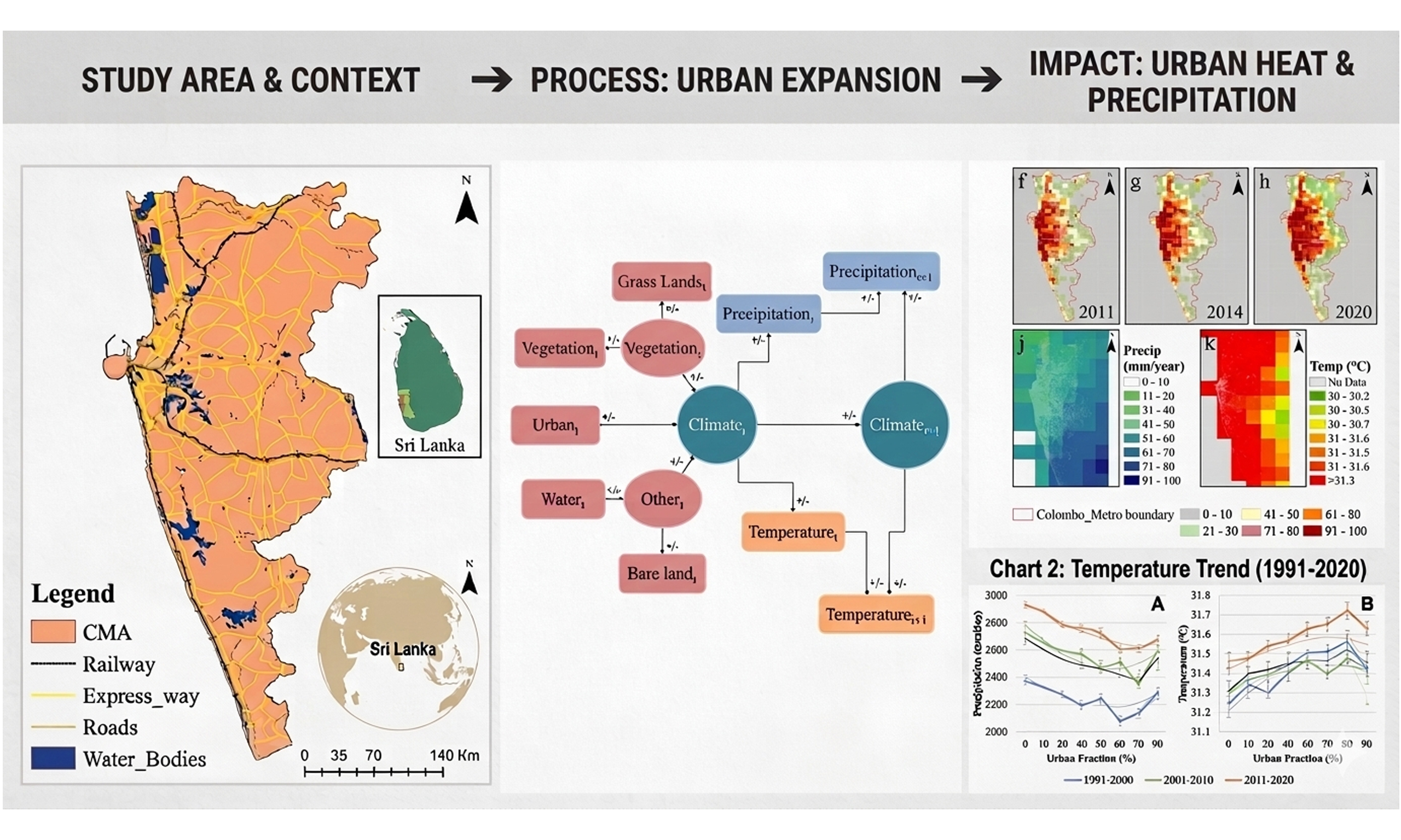
CMA has been selected as the case study [Figure 1] and is located in the Western Province of Sri Lanka. It has a population of 6.4 million, making it a densely populated area[36], and is one of the rapidly growing metropolitan belts in South Asia[37], featuring diverse climatic zones. CMA receives approximately 2,300 mm of rainfall annually[37,38]. It is a vital administrative, commercial, and industrial center, not only in the Colombo district but also in Sri Lanka. Rapid urbanization in CMA has resulted in significant environmental impacts, including global warming, altered climatic patterns, increased greenhouse gas emissions, and land-use changes[39]. These factors directly contribute to a significant rise in temperature and associated factors in urban areas[40]. The issues mentioned above pose significant challenges to urban sustainability and the environment. Unauthorized urbanization also has a major impact on climate change, affecting both local and regional climates. Small islands, such as Sri Lanka, are especially vulnerable to the effects of climate change due to their limited land area and resources. The CMA is a crucial monetary hub, so it is important to understand how urbanization in this region affects the broader environmental situation.
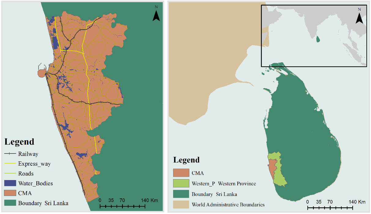
Figure 1. Study Area Map. The base map was derived from Natural Earth (https://www.naturalearthdata.com), a public domain resource with no copyright restrictions. CMA: Colombo Metropolitan Area.
Data used
To evaluate temperature and precipitation trends, this study used the CHIRPS (Climate Hazards Group InfraRed Precipitation with Station data) and CHIRTS (Climate Hazards Group InfraRed Temperature with Station data) datasets, which are widely recognized for their accuracy and reliability in representing climate variables. The accuracy and reliability of using CHIRPS and CHIRTS for the same study area have been validated by Fonseka et al.[38]. The dataset used in this study has proven reliability. In addition, Landsat imagery was employed for LULC classification. Landsat was chosen due to its long historical record, dating back to the early 1990s, and its relatively high spatial resolution of 30 m, making it suited for capturing urban expansion and vegetation changes over multi-decadal time periods. The combination of CHIRPS, CHIRTS, and Landsat enables a consistent and integrated assessment of LULC-climate interactions over the past three decades. The characteristics of the satellite products that were employed in this study are summarized in Table 1.
Gridded satellite products and characteristics
| Data | Resolution | Source |
| CHIRPS (Climate Hazards Group InfraRed Precipitation with Station) | 0.05° (5,550 m) | https://www.chc.ucsb.edu/data/chirps |
| CHIRTS (Climate Hazards InfraRed Temperature with Station data) | 0.05° (5,550 m) | https://www.chc.ucsb.edu/data/chirtsmonthly |
| Landsat Images | 30 m | http://glovis.usgs.gov/ |
Land cover classification and urban fraction calculation
The urban area information was obtained through the classification of Landsat images from 1992 to 2022 at four-year intervals, resulting in eight images that balance the need for temporal resolution with the availability of cloud-free scenes. The classification was performed using Random Forest classification in the Google Earth Engine (GEE) platform. For validation, ground truth data were obtained from high-resolution imagery from Google Earth Pro. To ensure the reliability of LULC classification, a thorough accuracy assessment was conducted for each classified image. These points were selected to represent known land cover types: urban areas, vegetation, and bare land across the study region and time periods. Standard accuracy metrics were calculated, including overall accuracy, producer’s accuracy, user’s accuracy, and the Kappa coefficient. Only classified maps with an overall accuracy greater than 80% and a Kappa value above 0.75 were retained for further analysis. This threshold was set to ensure high confidence in the spatial delineation of urban areas over time.
To assess the spatial distribution of urbanization, a uniform grid of 1.5 km × 1.5 km cells was overlaid across the study area. This resolution was chosen as a balance between spatial detail and computational efficiency, ensuring that localized urban expansion could be captured without introducing excessive noise from pixel-level misclassifications. Within each grid cell, the Urban fraction[41] was calculated by counting the number of urban pixels and dividing by the total number of pixels in the cell , as given in
where Nurban denotes the number of urban pixels and Ntotal denotes the number of total pixels within the respective grid. This gridded approach allowed for consistent spatial comparison across multiple time periods and minimized biases introduced by irregular administrative boundaries. The urban fraction was then categorized into 10 classes, with each class representing 10%. This classification threshold was selected to standardize the distribution of urban intensity and facilitate statistical modeling.
Diverse methods and application procedure
Climate data analysis: analyze the linear trend
To evaluate the relationship between urbanization and local climate dynamics, long-term precipitation and temperature data were obtained from the CHIRPS and CHIRTS datasets, respectively. Monthly values were averaged to produce annual averages, providing a clearer view of long-term trends while smoothing out short-term fluctuations. Subsequently, the relationship between urban fraction and annual temperature and precipitation trends was analyzed. Each grid cell was linked to the corresponding urban fraction calculated from the classified Landsat data. To analyze the evolution of urban-climate interactions over time, both urban fraction, temperature, and precipitation were summarized into three decades: 1991-2000, 2001-2010, and 2011-2020. This stratification provides a structured approach to evaluate changes over time and facilitates an understanding of the evolution of urbanization and its potential effects on climate parameters.
Precipitation-temperature relationship analysis
The CHIRPS and CHIRTS data from 1980 to 2020 were used to study the precipitation-temperature (P-T) relationship and to further explore how urbanization may affect extreme precipitation patterns in relation to temperature. The analysis was divided into two equal time windows: data from 1980 to 2000 were used as F20Y (first 20 years), and data from 2000 to 2020 were used as L20Y (last 20 years). This split allows for the comparison of historical and more recent urban-climate dynamics, enabling assessment of how the intensification of urban land use may have altered precipitation responses under warming conditions. The methodology follows the framework proposed by Landerink and Meijgaard[42], where temperature bins were defined using a sliding 2 °C window, updated every 1 °C, to prevent the selection of odd or even bin limits[41,43,44]. Within each bin, the 95th percentile of daily precipitation values was calculated to represent extreme precipitation. This high percentile threshold was chosen to emphasize rare but impactful events such as flash floods, which are of particular relevance for urban planning and disaster risk management.
To isolate potential differences between urban and non-urban areas, the P-T relationship was calculated separately for grid cells with high urban fraction (≥ 70%) and those with low or no urbanization (≤ 10%). Every urban or other grid was taken into account independently while building the P-T relationship. The Two-sample Kolmogorov-Smirnov (K-S)[41,44] test was performed for the urban-other difference in the P-T relationship and expressed as follows:
where Dn,m represents the K-S test statistic, sup stands for the supremum function and Fu,n and Fr,m, respectively, are the empirical distribution functions of the precipitation samples in the cities and the countryside at a certain temperature bin. The null hypothesis, which states that the distribution of precipitation samples in urban and other areas is the same, is rejected at level α for large samples. The critical value (Dn,α) is given in
where n and m are the numbers of precipitation samples in urban and other areas, respectively. At a 5% significance level, the constant c(α) in Equation 3 takes the standard tabulated value of 1.358 for a two-sample Kolmogorov-Smirnov test. This constant is used to calculate the critical threshold for rejecting the null hypothesis. To address potential sources of uncertainty, data preprocessing steps including quality screening of satellite data (e.g., removing missing values, averaging over full-year observations), and the use of robust non-parametric tests (e.g., K-S) that do not assume normality were utilized. However, this analysis does not explicitly control for larger-scale climate variability [e.g., El Niño-Southern Oscillation (ENSO), Indian Ocean Dipoles (IOD)], which may influence precipitation trends at decadal scales. While these factors are acknowledged as limitations, the spatial design of the study, focusing on comparative analyses within a fixed geographic region, helps to minimize their confounding effects.
Structural equation model analyses
The influence of LULC, including urbanization, on local climate was analyzed using a SEM[30,45]. SEMs are effective at testing causal hypotheses with empirical data, offering unstandardized interaction values similar to partial regression coefficients for direct interpretation, alongside standardized coefficients that highlight a predictor's unique contribution to explaining variance in a response variable[45]. SEMs are a commonly utilized approach in ecological research, enabling researchers to investigate the effects of variables on one another through direct, indirect, and mediator interactions[45,46]. One of their strengths is their ability to address multicollinearity issues, positioning them as a superior alternative to traditional multivariate regression in certain contexts[30,46].
Each grid was treated as a sample in the study, covering an area of 1.5 km2. Three classifications were utilized for each 10-year period. We considered the land use classifications on the grid as exogenous observed variables, while the annual average temperature and precipitation on the grid were treated as endogenous observed variables. A latent climate construct was introduced to capture underlying variability in climate, with temperature and precipitation defined as its observable indicators. This latent construct allows the model to account for joint variations in these variables that may not be fully explained by each metric alone. Causal paths were hypothesized from LULC variables (urban, vegetation, bare land) to the latent climate variable. This assumption is grounded in prior empirical and theoretical work, ultimately influencing local temperature and precipitation regimes. The conceptual model structure is illustrated in Figure 2, with arrows representing hypothesized causal relationships based on urban climate literature. Broader climatic variability was not explicitly modeled but is partially captured through the long-term average climate values, reducing the effect of short-term anomalies. This model was applied in three separate decades. Figure 2 introduces the foundational hypothesis of our SEM analysis, which presents conceptual bidirectional relationships.
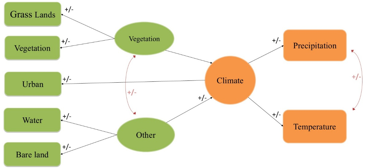
Figure 2. Foundational hypothesis of SEM Model. SEM: structural equation model.
Dynamic structural equation modeling
This study employed a DSEM to investigate the interdependencies between land use and climatic data over time and to explore temporal dependencies. This approach enables analysis of the complex inter-relationships between land use patterns and climate variables across different decades[47]. This modeling approach is particularly suited for analyzing time-ordered data, allowing researchers to explore how changes in land use influence climate over time and vice versa. By incorporating dynamics into the SEM framework, the DSEM captures both direct and indirect effects, as well as the temporal interdependencies between variables. Both SEM and DSEM were applied using the R statistical package. Figure 3 introduces the foundational hypothesis of our dynamic SEM analysis.
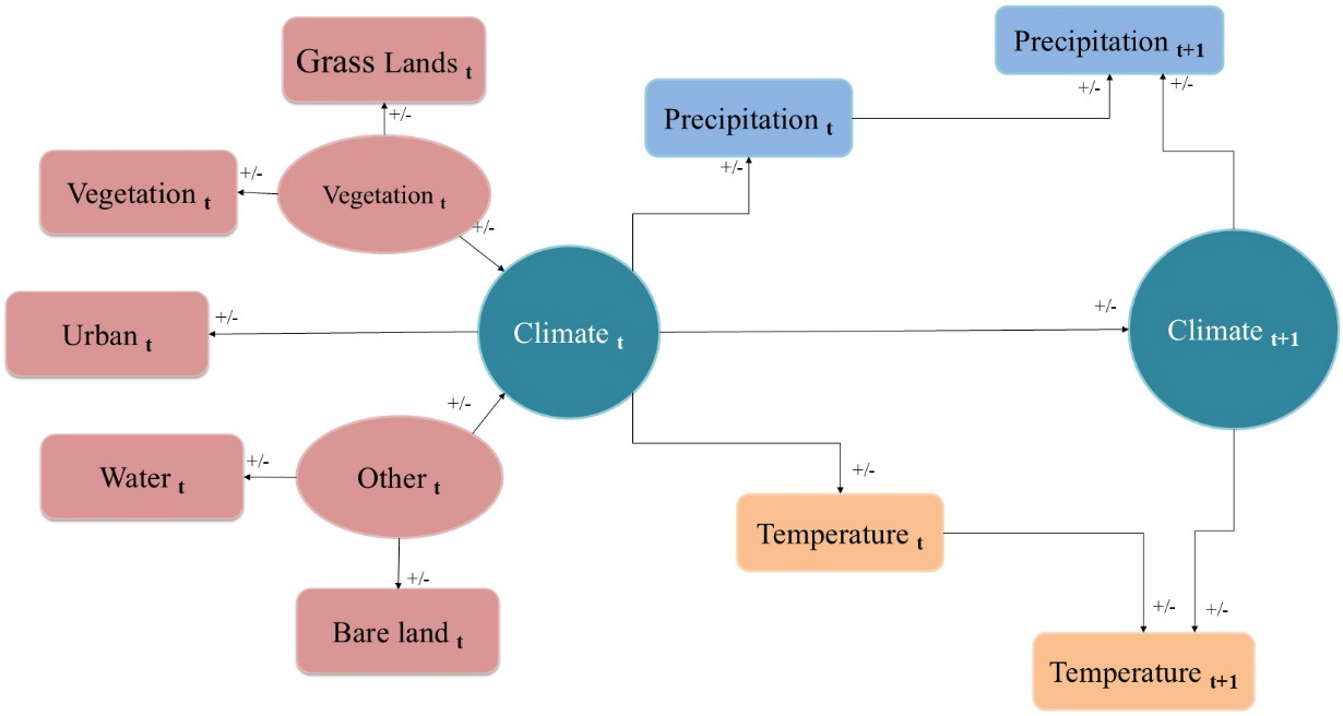
Figure 3. Foundational hypothesis of Dynamic SEM Model. SEM: structural equation model.
RESULTS
Urban area classification
After classification, the urban areas were extracted using classification results, and the urban fraction for each year was calculated per grid using Equation 1 and is shown in Figure 4.
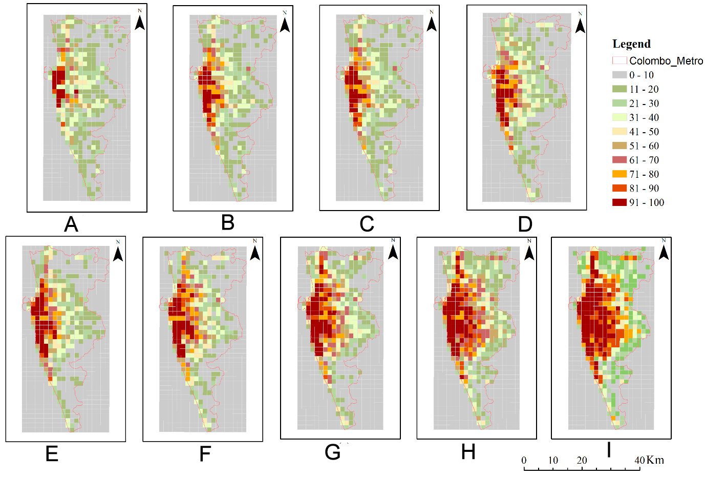
Figure 4. Urban Fraction of Colombo Metropolitan (A) 1990 (B) 1994 (C) 1998 (D) 2002 (E) 2006 (F) 2010 (G) 2014 (H) 2018 and (I) 2022.
Over the 30-year period, a noticeable increase in the number of pixels classified as urban can be observed as depicted in Figure 4. This suggests that the extent of urban areas has expanded considerably over time. The regions with high urban density, those with an urban fraction above 50%, have become more pronounced. As depicted in Figure 1, the western border of the CMA is the Indian Ocean, and urban expansion is densely concentrated along the coastline[31], with potential for growth inland. By 2020, areas with an urban fraction of 90% or higher, likely representing highly developed and densely populated regions[31], had emerged. Although the urban fraction is increasing, it does not necessarily indicate whether CMA is experiencing urban development or sprawl. However, a study by Fonseka et al.[31] suggested that the study areas are characterized by unplanned development, inadequate infrastructure, loss of green spaces, and increased environmental stress associated with unhealthy urbanization.
Climate data analysis
Analyze the linear trend
The average temperature and precipitation of each grid were summarized and plotted in Figure 5.
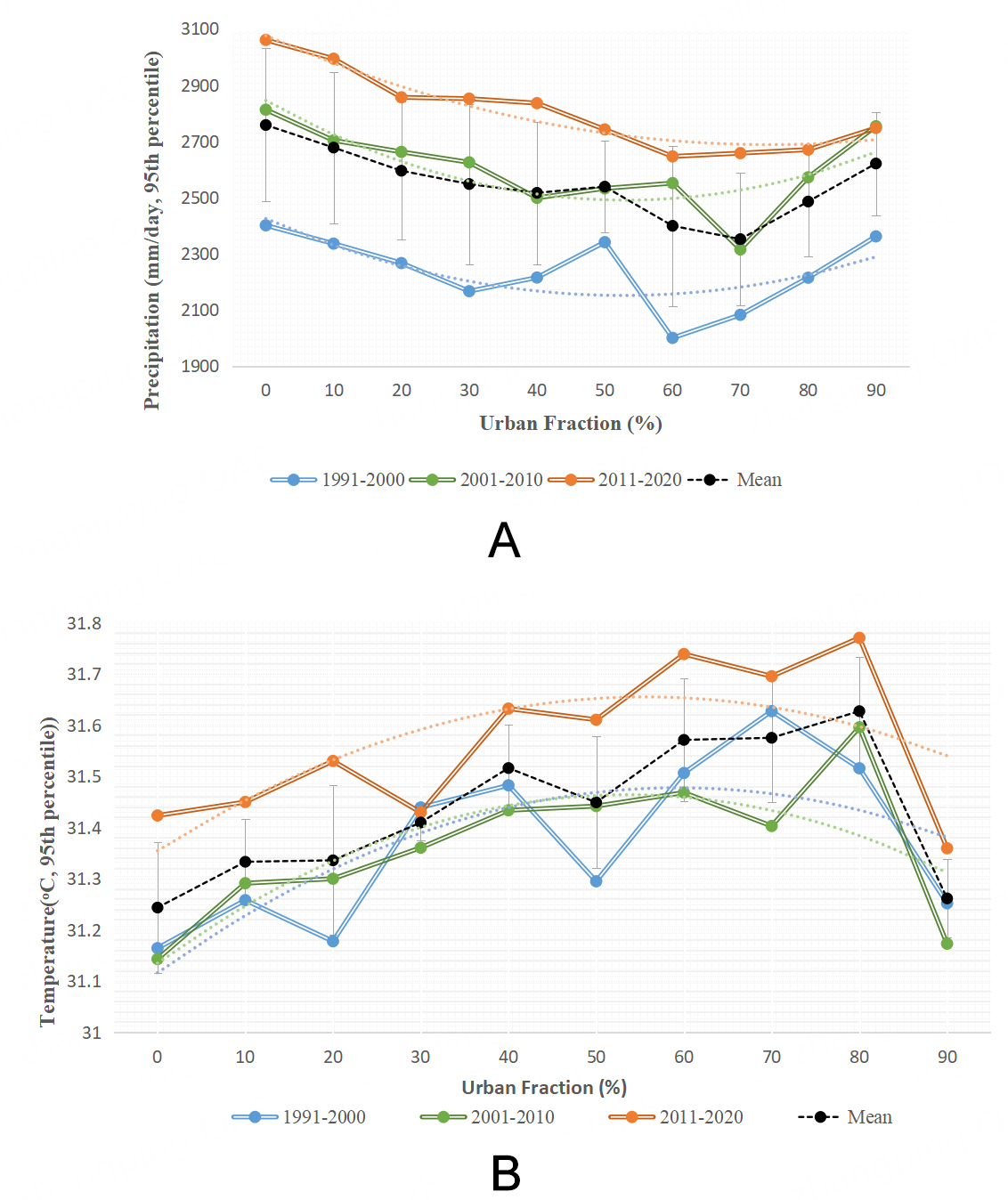
Figure 5. (A) Urban Fraction versus Precipitation (B) Urban Fraction versus Temperature.
Figure 5A presents the precipitation versus urban fraction in three decades. It further presents a point at which the urban fraction reaches approximately 58%, where precipitation decreases and then begins to increase again in each decade. This could be interpreted as a U-shaped relationship between urban fraction and precipitation. The curvature of the relationship varies by decade, with the strongest U-shape observed in 1990-2000 (curvature coefficient a = 0.203), followed by 2000-2010 (a = 0.160), and a flatter curve in 2010-2020 (a = 0.099), indicating a weakening sensitivity of precipitation to urban expansion over time. Corresponding minimum precipitation values increased from 1,990 mm in the 1990s to 2,689 mm in the 2010s.
The U-shaped precipitation trend can be explained by the effects of urbanization on local moisture and atmospheric processes. In areas with lower urban fractions, the replacement of vegetation with impervious surfaces (e.g., asphalt) likely reduces evapotranspiration and moisture availability. During this stage, the urban heat island (UHI) effect may increase temperatures, but it does not immediately lead to higher rainfall[48]. However, beyond a certain threshold of urbanization, the intensified UHI effect can drive stronger updrafts of warm air, promoting convective cloud formation and potentially increasing precipitation[49]. Human activities in urban areas may also release aerosols and moisture, which might further modulate cloud microphysics, being possible drivers of precipitation changes in urban environments[50]. Nevertheless, our dataset does not allow us to separate the role of local-scale mechanisms from broader regional circulation; therefore, the observed U-shape should be interpreted as a statistical pattern rather than a direct attribution of causality[51].
On the other hand, as the urban fraction increases to 57% [Figure 5B], the average temperature reaches a minimum, and then begins to rise up to about 70%-80%, after which it shows a decline at the highest urban fraction levels. This pattern indicates an inverted U-shaped relationship between urban fraction and temperature. Specifically, the turning points - the lowest average temperatures - occur consistently near an urban fraction of 56.7% in 1990-2000 (31.30 °C), 57.0% in 2000-2010 (31.42 °C), and 57.4% in 2010-2020 (31.57 °C), suggesting a stable temperature response threshold across decades. In terms of shape, the strength of this inverted U-shaped pattern varies slightly, with curvature coefficients of 0.89 in 1990-2000, 0.71 in 2000-2010, and 0.95 in 2010-2020, indicating increasing sensitivity of temperature to urban expansion in the most recent decade[51]. Inverted U-shaped relationship between urban fraction and temperature reflects the balance between cooling effects from green infrastructure and increased heat absorption from the impervious surface. At lower urban densities, vegetation can help moderate local temperatures[51]. However, with the increased urban density, these cooling effects may be offset by the UHI phenomenon, where impervious surfaces and reduced vegetation lead to greater heat absorption and re-radiation, raising local temperatures[51]. Research on urban morphology has shown similar trends, with urban density and land surface temperature being closely linked[52]. Overall, these trends suggest the complex relationship that underscores the dynamic interactions between urbanization, temperature, and precipitation.
P-T relationship analysis
The average temperature, as well as the 95th percentile of temperature and precipitation for the first 20 years (denoted as F20Y) and the last 20 years (denoted as L20Y), were computed. We observed abrupt changes rather than gradual changes.
The regional distribution of mean temperatures during F20Y and L20Y is shown in Figure 6A and B, respectively, while the distribution of extreme temperatures for the same periods is presented in Figure 6C and D. The 95th percentile was used to identify extreme values. Both average and extreme temperatures increased in L20Y compared to F20Y, indicating overall warming. The urban areas exhibit greater mean and extreme temperature values (first and third columns) than their “other” counterparts, consistent with the expected consequences of UHI. Built-up areas are visible in the overlay on the temperature maps. Overall, the upward trend in temperature between F20Y and L20Y provides evidence of warming, with the gap more pronounced in urbanized areas compared to other regions.
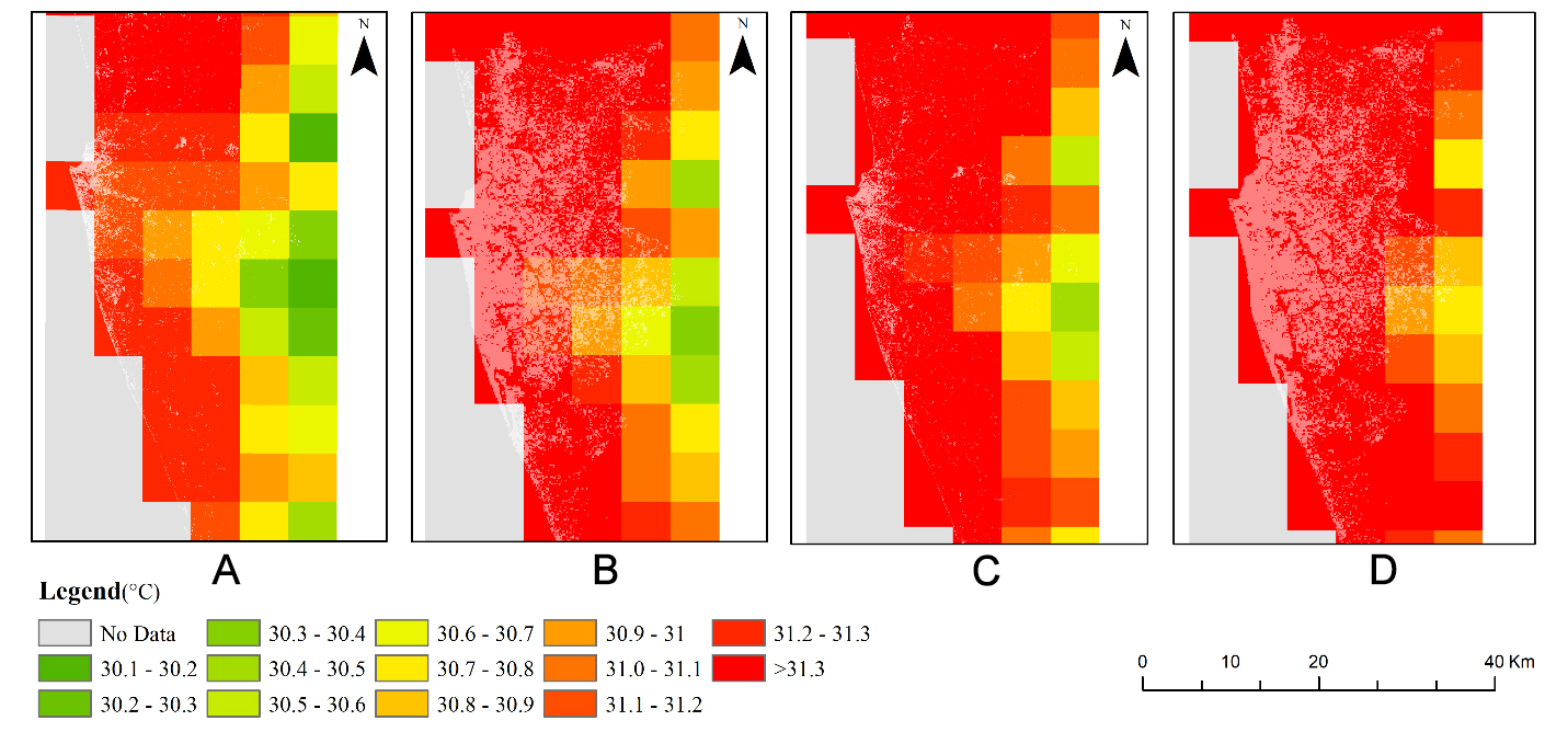
Figure 6. (A) Average of F20Y Temperature; (B) Average of L20Y Temperature; (C) 95th Percentile of F20Y Temperature; (D) 95th Percentile of L20Y Temperature.
The mean precipitations are shown in Figure 7A and B, while extreme precipitations are displayed in Figure 7C and D. In contrast to the temperature patterns depicted in Figure 6, no maximum precipitation scenarios were observed in urban areas. The highest values of both mean and extreme precipitation are observed to be away from the high urban regions of CMA. However, it can be seen that the precipitation has increased from F20Y to L20Y. This rise may be associated with the expansion of urban infrastructure and its associated potential climatic impacts, such as the UHI effect, which can enhance local convection and cloud formation, finally leading to increased precipitation[41,49]. The distinction is more apparent when analyzing extreme precipitation (95th percentile). The intensification of extreme precipitation over urban areas may reflect stronger energy and moisture dynamics in urban settings[44,53], leading to more intense rainfall events. These findings highlight important considerations for infrastructure development and climate adaptation strategies in the urban areas of the CMA.
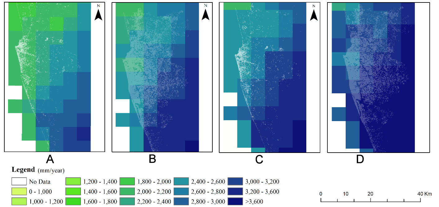
Figure 7. (A) Average of F20Y Precipitation; (B) Average of L20Y Precipitation; (C) 95th Percentile of F20Y Precipitation; (D) 95th Percentile of L20Y Precipitation.
Urban effects on P-T relationship
The aforementioned findings imply that variations in temperature and precipitation in the study region are more noticeable at their extremes. In this section, the relationship between extreme precipitation and temperature is quantitatively examined by constructing the P-T relationship, including the time-mean relationships in the urban and other areas. The extreme precipitation scaling in relation to the mean surface air temperature is depicted in Figure 8, showcasing separate variations for urban and other regions.
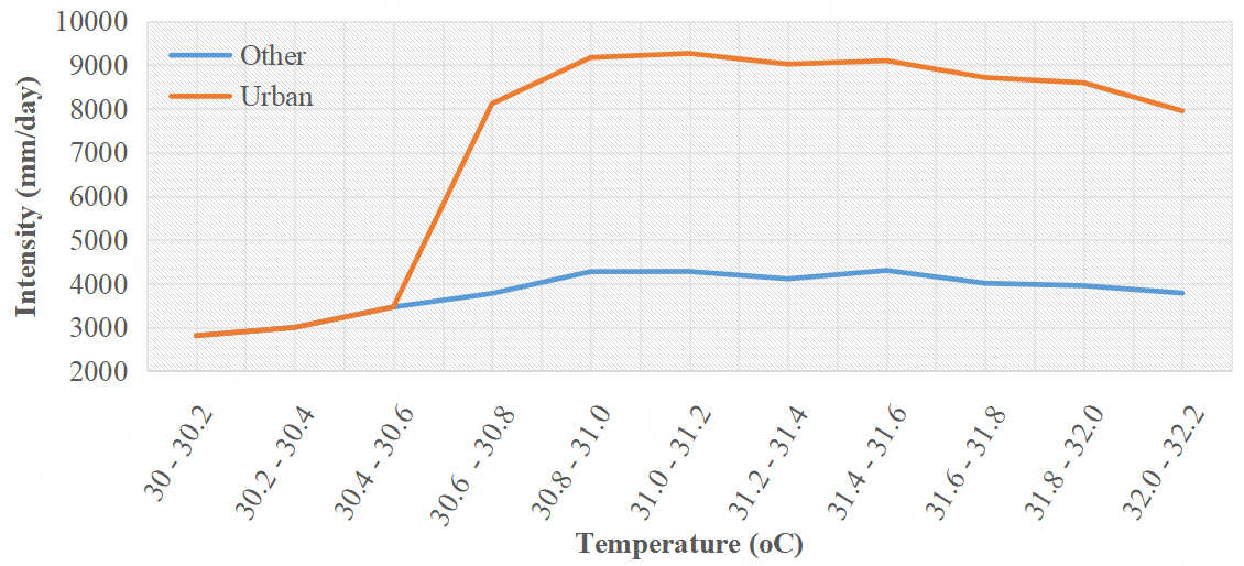
Figure 8. The 95th percentile of daily precipitation (mm/day) as a function of surface air temperature (°C) (i.e., P-T relationship) in the urban and other areas.
When aggregating all urban or other grids, only the extreme precipitation - the 95th percentile of precipitation - is taken into account in each temperature bin. The “Urban” line shows a clear peak-like structure[41]. Precipitation increases with temperature up to a certain point termed the “breaking point”, after which it levels off[53]. This peak suggests that there is an optimal temperature range for precipitation in urban areas, beyond which higher temperatures do not lead to more precipitation[41]. This could be due to various factors, such as the UHI effect, which can affect local weather patterns[53,54]. The "Other" line remains relatively flat and lower in value compared to the “Urban” line. This indicates that the precipitation does not vary much with temperature and is consistently lower than in urban areas within the given temperature range.
Super-Clausius-Clapeyron (CC) scaling refers to a rate of increase in extreme precipitation intensity with temperature that is higher than what would be expected from the traditional CC[55] relationship, which predicts a 7% increase in atmospheric water vapor holding capacity with each 1 °C rise in temperature[55]. In the scenario described, extreme precipitation intensity increases with temperature until a breaking point and then decreases beyond it. Up to the breaking point temperature, the increase in precipitation intensity might follow a super-CC scaling, steeper than the traditional CC relationship[41]. This could be interpreted as the precipitation intensity increasing by 7% per degree Celsius for each degree of temperature rise above the expected value. After reaching the breaking point, the trend reverses, possibly due to atmospheric dynamics[55,56] that limit further increases in moisture[55] or changes in storm structure and dynamics[53] that become dominant at higher temperatures.
Decadal extreme event trends
Figure 9 illustrates the decadal proportions of different hazard events, as reported by the Disaster Management Centre of Sri Lanka. A notable increase in urban floods and landslides was observed during the 2000-2010 period, suggesting a shift in hazard types associated with intensified urbanization. Flooding remains the most frequent event type throughout the study period, with a substantial spike recorded in the 2000-2010 decade, coinciding with rapid urban growth in the CMA. These events are typically associated with altered surface hydrology, reduced infiltration capacity, and increased runoff, resulting from the expansion of impervious surfaces due to unplanned urban development.
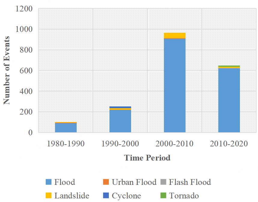
Figure 9. Trends in Hazard Events Over Decades.
This pattern aligns with findings from the above P-T relationship analysis. The results suggest a non-linear, peak-like relationship between surface air temperature and extreme precipitation in urban areas, where precipitation intensity increases with temperature up to a “breaking point,” beyond which it declines. The observed decline in extreme rainfall during the 2010-2020 period, despite continued urban warming, reflects this climatic tipping point. When urban temperatures exceed this threshold, convective uplift can weaken, and the atmosphere may hold more moisture without releasing it as precipitation, resulting in fewer, but potentially more intense or irregular, rainfall events.
In addition, a comparison between the 1980-1990 period and later decades shows a marked increase in hazard events, underscoring the role of urbanization in amplifying local climate extremes. However, it should be acknowledged that these changes are influenced not only by local anthropogenic activities but also by broader regional climatic phenomena, which will be briefly considered in the following section to provide additional context.
Relationship between ENSO, IOD, and climate extremes
Figure 10 compares the annual 95th percentile values of temperature and precipitation in the CMA with regional climate indices. The indices include ENSO, obtained from https://www.cpc.ncep.noaa.gov/, and IOD, obtained from http://www.bom.gov.au/, for the period 1980-2020 (accessed on May 20, 2025). ENSO and IOD exhibit significant interannual variability, with clear peaks and troughs corresponding to the known El Niño and IOD events. In contrast, temperature extremes show a gradual upward trajectory over time. This long-term increase in temperature may be influenced by rapid urbanization and the intensification of the UHI effect, although other regional factors could also play a role. The pronounced temperature extremes and precipitation anomalies observed in the CMA, even during ENSO neutral years, suggest that local anthropogenic factors may contribute to the observed long-term climate extremes.
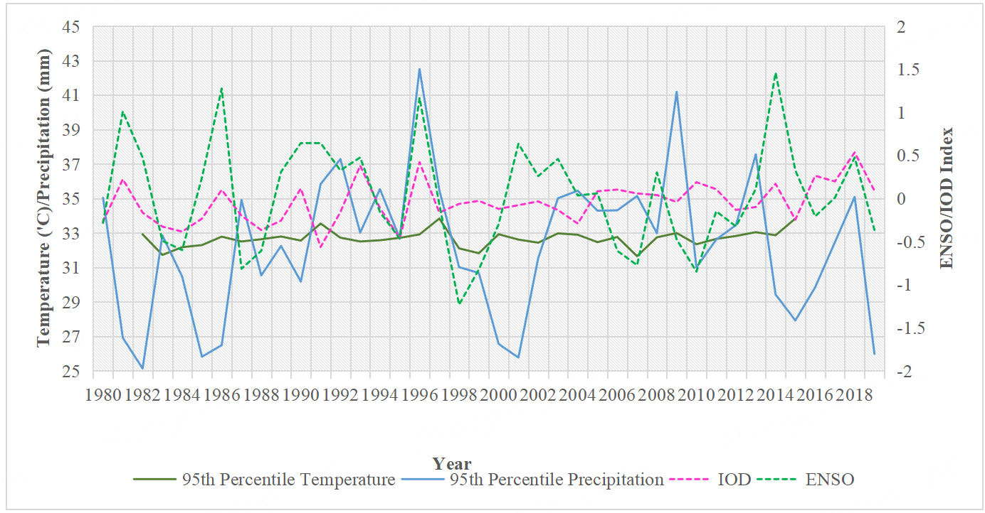
Figure 10. Temporal trends of ENSO, IOD, and corresponding changes in 95th percentile temperature and precipitation. ENSO: El Niño Southern Oscillation; IOD: Indian Ocean Dipoles.
In contrast, precipitation extremes exhibit a nonlinear pattern, characterized by sharp year-to-year fluctuations rather than a consistent trend. Some of these fluctuations appear to align with ENSO and IOD phases, supporting the role of these teleconnections in short-term climate variability. However, in more recent years, extreme precipitation appears to decline despite rising temperatures. This pattern is consistent with the P-T relationship identified in this study, which indicates a “breaking point” beyond which further temperature increases may suppress precipitation. One possible explanation is urban-induced atmospheric stabilization and reduced convective activity, though further investigation is needed. In summary, ENSO and IOD likely contribute to episodic and spatially broad variability, while urbanization may play an increasing role in shaping localized climate extremes in the CMA[38].
Structural equation model analyses
The objective of this research is to quantify the impacts of LULC change, especially urbanization, on the regional climate. The results of the three-decade analysis are summarized in Figure 11.
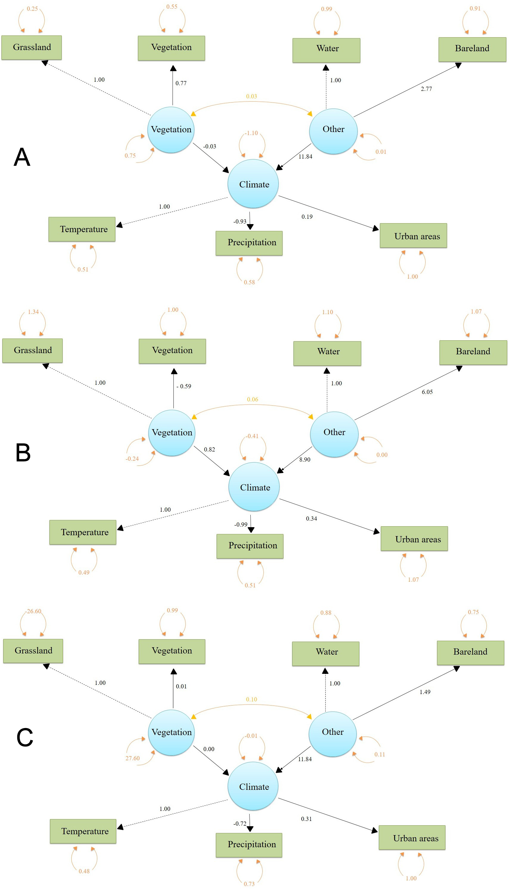
Figure 11. Structural Equation Model results for (A) 1991-2000 (B) 2001-2010 and (C) 2011-2020.
The structural model displays that all the parts of the vegetation area, urban area, and other areas are associated with regional climate variables. As illustrated in Figure 11, the model shows that other areas, which mainly include water and bare land, have positive effects on regional climate change. Bare land emerged as a particularly strong contributor, as the “Other → Climate” pathway showed the largest standardized coefficients: 0.42 in 1990s [Figure 11A], 0.48 in 2000s [Figure 11B], and 0.51 in 2010s [Figure 11C]. Among the two representatives of the “Other” category, water remains constant, and therefore, the impact of bare land on climate is considerable. Furthermore, bare land use has changed significantly over the past three decades.
The urban → climate pathway also showed a steady increase in influence, with standardized coefficients of 0.27 in 1990s [Figure 11A], 0.34 in 2000s [Figure 11B], and 0.39 in 2010s [Figure 11C]. This indicated an intensification of urban contribution to climate variability, likely linked to expanding impervious surfaces and anthropogenic heat release. However, we avoid claiming direct causality, as the model captures statistical associations rather than mechanistic processes. Conversely, the vegetation → climate pathway declined over time (0.36 to 0.22), consistent with observed vegetation loss and diminishing green cover in urbanizing regions. These results suggest that as urban areas expand and vegetation is lost, the landscape’s cooling and moisture-regulating capacity weakens. Additionally, a small but consistent climate → urban feedback was detected (coefficients ~0.10–0.13), suggesting that climatic shifts may also influence urban growth patterns, possibly through changes in development pressures or infrastructure responses to climate risks. To evaluate model adequacy, the main goodness-of-fit indices for each period are summarized in Table 2. For the 1990s, the model achieved a reasonably good fit [Comparative Fit Index (CFI) = 0.87, Tucker-Lewis Index (TLI) = 0.86, Root Mean Square Error of Approximation (RMSEA) = 0.06, Standardized Root Mean Square Residual (SRMR) = 0.04]. Model performance improved in the 2000s (CFI = 0.92, TLI = 0.88, RMSEA = 0.08, SRMR = 0.02). In the 2010s, the CFI remained acceptable (0.92), though the TLI weakened (0.84) and RMSEA was higher (0.18), partly offset by a very low SRMR (0.01).
SEM model fit summary
| Period | Observations | Chi-square (df) | CFI | TLI | RMSEA | SRMR |
| 1990 to 2000 | 100 | 40.722 (11) | 0.871 | 0.864 | 0.064 | 0.037 |
| 2000 to 2010 | 112 | 52.135 (11) | 0.922 | 0.878 | 0.083 | 0.024 |
| 2010 to 2020 | 106 | 48.221 (11) | 0.915 | 0.838 | 0.179 | 0.012 |
Overall, although some indices, particularly TLI and RMSEA in later years, fall below ideal thresholds, others (CFI, SRMR) consistently indicate acceptable performance. This suggests that the SEM provides a broadly valid representation of land-climate interactions in the CMA. The observed weaknesses do not undermine the main conclusions, though results should still be interpreted with an awareness of these limitations.
While the conceptual models [Figures 2 and 3] hypothesize both bidirectional and multivariate interactions among land-use types and climate variables, the empirical models [Figure 11] reveal a more selective set of statistically significant paths. For instance, the bidirectional relationship between temperature and precipitation proposed in Figure 2 was not strongly supported in the SEM results [Figure 11], where directional pathways (e.g., Urban → Climate) dominated. Similarly, while Figure 3 hypothesizes strong temporal feedback between climate variables across decades, the DSEM results [Figure 12] show only modest cross-lagged effects, such as Climatet (climate variable at time t) → Climatet+1 (climate variable at time t+1). The weakening path coefficients from vegetation and other land types in later decades also contrast with the uniformly weighted conceptual paths. These discrepancies suggest that while the hypothesized framework is comprehensive, empirical dynamics are more context-sensitive, particularly under the tropical island context of the CMA.
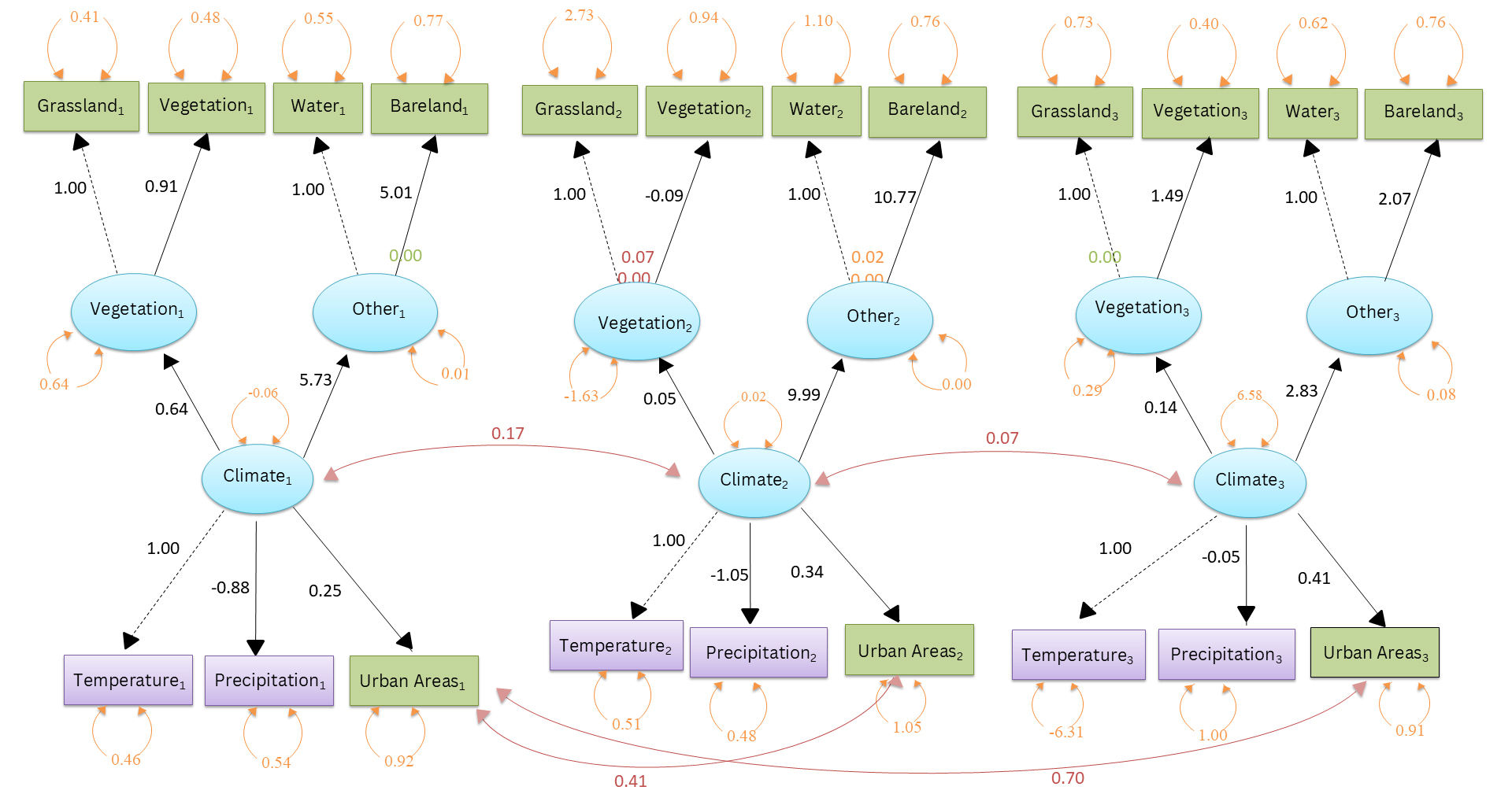
Figure 12. Dynamic Structural Equation Model Results.
Dynamic structural equation modeling
To investigate the interrelationships between decadal land use and climate data, a DSEM was used. Results from the fitted data to the dynamic model are presented in this section in Figure 12. Using the state-space formulation, the parameter matrices have been estimated by maximizing the likelihood function using the Kalman filter[43].
The results from the DESM [Figure 12] illustrate the complex interactions between various land-use categories and climate variables over three time periods. The model indicates that the interaction between vegetation cover and the latent “Climate” construct fluctuates over time. As depicted in Figure 12, in the early period (1990-2000), Vegetation1 → Climate1 shows a path coefficient of 0.64, indicating a relatively strong contribution. However, this influence decreases across decades, dropping to 0.07 in 2000-2010 and further to 0.14 in 2010-2020, suggesting a weakening role of vegetation in regulating local climate patterns. Both temperature and precipitation contribute significantly to the measurement of Climate in each period. Cross-lagged paths between decades (e.g., Climate1 → Climate2 = 0.17 and Climate2 → Climate3 = 0.07; Figure 12) further reflect modest continuity in climate dynamics across time, reinforcing the assumption of gradual environmental shifts. The fluctuating impact of temperature on urban areas shows significant variability in its influence over time. Urban areas consistently exert a strong influence on the climate system, particularly in the later time periods. As shown in Figure 12, urbanization has increased significantly between the first and third periods, suggesting rapid land-use change in the region. Such land-use change reduces green cover, increases impervious surfaces, and thereby intensifies urban heat effects. The model also suggests how urban expansion influences the water and vegetation balance, potentially amplifying microclimatic changes. Based on this dynamic model, the local situation seems to depict ongoing urbanization and its impact on climate variables, particularly precipitation and temperature. The transition from natural land covers (grasslands, vegetation) to urban areas has altered local microclimates, leading to increased temperatures and changed precipitation patterns, likely contributing to increased climate variability. This is especially significant in urban regions where vegetation cover reduction intensifies urban heat effects. Additionally, the weakening role of natural ecosystems such as grasslands and vegetation may reduce climate resilience in the region, making the area more vulnerable to extreme climate events.
To assess model adequacy, the main fit indices across decades were summarized: (1) 1990-2000: CFI = 0.871, TLI = 0.864, RMSEA = 0.064, SRMR = 0.037, suggesting a moderately acceptable fit; (2) 2000-2010: CFI = 0.922, TLI = 0.878, RMSEA = 0.053, SRMR = 0.024, suggesting improved fit approaching adequacy thresholds; (3) 2010-2020: CFI = 0.915, TLI = 0.838, RMSEA = 0.049, SRMR = 0.012, showing mixed results with strong CFI/SRMR but weaker TLI and RMSEA. While some indices (CFI, SRMR) fall within acceptable ranges, others (TLI, RMSEA) highlight weaknesses, particularly in later decades. These results suggest that the model captures plausible causal relationships but should be interpreted with caution. The structural consistency across decades nevertheless provides meaningful insight into the evolving influence of land-use changes on climate.
DISCUSSION
The urban expansion of the CMA has been examined by various studies, including those by Ranagalage et al.[37]. Fonseka et al.[38], and Subasinghe et al.[39], which demonstrate that the area is undergoing extensive urbanization without proper management strategies. Therefore, the impact of local climate variability requires careful attention. This study first analyzes the variability of temperature and precipitation in relation to urban fraction. Across all three periods, precipitation initially decreases as the urban fractions increase, while temperature generally rises with increasing urbanization, although not in a strictly linear manner. A clear UHI effect is evident. The results indicated that urbanization initially tends to negatively affect precipitation. However, the rebound in precipitation beyond a certain threshold may suggest more complex atmospheric interactions[44,48]. The rising temperatures in recent decades imply an intensification of urban warming, possibly driven by denser construction and broader climate change impacts within the CMA. Similar quantitative analyses regarding the contribution of LULC change to variations in climatic factors such as precipitation and temperature are reported in studies by Chu et al.[19], Qian et al.[44], and Cao et al.[20]. However, Laux et al.[23] presented a situation with no significant signal for precipitation change while a clear temperature trend is observed.
Drawing upon the analysis conducted throughout this research, dynamics of urbanization employ a significant and apparent influence on local climate patterns, distinct from other land-use types[57]. The DSEM revealed how vegetation, urbanization, and other factors dynamically interact and influence the climate over three consecutive decades. Key findings indicated that urban expansion, marked by the increase in urban pixels, particularly in the Colombo Port and Rathmalana areas, has played a critical role in shaping climate trends. The rising intensity of urban development has been directly correlated with alterations in temperature and precipitation patterns, underlining the UHI effect as a crucial factor in modifying local climate dynamics[48,44]. The unique contribution of urbanization to climate change was underscored by the quantitative investigation of the P-T relationship, which revealed that extreme urban precipitation patterns deviate from those in other settings. This demonstrates that urban areas, through various anthropogenic activities and alterations in land surface properties[19], contribute distinctly to the hydrological cycle and temperature regulation.
Importantly, the SEM results provided a quantitative perspective that urbanization showed a consistent positive association with temperature and a weaker negative association with precipitation. These results suggest that urbanization explained roughly 10%-20% of the variance in temperature trends and 5%-10% of the variance in precipitation trends, depending on the period. While these estimates should be interpreted with caution, given the modest model fit, they strengthen the evidence that urbanization has been a substantial driver of local climate change in the CMA.
In mid-latitude regions, a peak-like (or hook-like) structure in the P-T relationship is typically observed, where precipitation intensity increases with temperature up to a certain threshold and then decreases sharply[58]. Similar peak structures have been observed in countries and regions such as Australia, the Indian Monsoon zone, and other mid-latitude areas[58,59]. However, in the case of the CMA, the peak is less pronounced. Nevertheless, comparable findings have been reported in other studies, including those by Oh et al.[41], Wang et al.[56], Zeder and Fischer[60], and Jing et al.[8]. In contrast, some researchers argue that there is spatial variation in the P-T scaling rate before reaching the peak, and the role of seasonality in shaping this relationship has also been highlighted[44]. The SEM and DSEM have revealed how vegetation, urbanization, and other factors dynamically interact and influence the climate over three consecutive decades. In this study, SEM was employed due to its applicability in environmental research, as demonstrated in studies by Krivoguz et al.[30]. Nevertheless, the literature showcases only a few studies that have examined the impact of urbanization on climate indicators using SEM[30,57].
Wang et al.[58] applied structural modeling in 2015 to study the impacts of land use change on regional climate. The findings of this research align with those of the current study, demonstrating that vegetation areas, urban areas, and surrounding regions can all impact regional climate to varying extents. Notably, vegetation areas exhibit a negative relationship with regional climate change. However, previous studies clearly indicate that the decrease in vegetation resulting from deforestation and urbanization contributes to increases in temperature and precipitation in low-latitude areas[52].
It is notably evident that the rapid urbanization characteristic of modern development showcases profound implications for the climate of CMA. According to Fonseka et al.[38], the climate of the CMA has undergone noticeable transformations between 1980 and 2020, with urbanization identified as a key driver behind these shifts. The observed rise in temperature and the altered precipitation patterns reflect the cumulative effects of land cover changes, anthropogenic heat release, and reduced vegetation, all of which are inherent consequences of unplanned urban growth.
This local climate transformation, especially in small islands, must be understood not in isolation, but within the broader global framework of sustainability and resilience, particularly as it relates to the United Nations SDGs. Goal 11: Sustainable Cities and Communities, which emphasizes the importance of making urban areas inclusive, safe, resilient, and sustainable. This is very important in the context of CMA. As urban sprawl continues and infrastructure struggles to keep pace, the region faces challenges such as increased heat stress, urban flooding, and diminished air quality. Moreover, Goal 13: Climate Action focuses on strengthening resilience and adaptive capacity to climate-related hazards. As a coastal urban hub in a small island developing state (SIDS), the CMA is especially vulnerable to the dual threats of climate change and sea level rise. The knowledge garnered from this research holds significant potential for informing policy and guiding sustainable urban planning practices.
STUDY LIMITATIONS
This study has several limitations as follows:
1. The goodness-of-fit results in the SEM were varied in some periods. These results reflect the complexity of representing dynamic land-climate interactions with the currently available variables. Although additional data could potentially enhance model performance, the present analysis still provides meaningful insights into the evolving influence of urbanization and land-use change on local climate. The model should therefore be interpreted as an exploratory framework that highlights key interactions rather than a final predictive tool. Developing models with smaller temporal gaps may offer further insights into short-term dynamics of these interactions.
2. Although parameterizing urban land surfaces is challenging due to their heterogeneity and small spatial extent compared to typical climate and land cover datasets, our model attempts to capture these dynamics by incorporating urban indicators within the structural framework.
3. Comparative studies simulating the urbanization process in regional climate models remain limited in allowing for comparisons and conclusions regarding the findings. This research primarily focused on satellite images, where the constraints of spatial resolution significantly impact the results with uncertainties, but still provide valuable insights into land-use-climate interactions.
Despite the unavailability of ground data, the satellite data still provides valuable insights. In the context of sustainable development for small islands, these limitations highlight the urgent need for comprehensive studies that incorporate diverse data sources and methodologies. As small islands face unique vulnerabilities to climate change, understanding the impact of urbanization becomes essential for developing effective sustainability strategies. Incorporating the influence of regional climatic events into this type of analysis could further enhance the investigation of results, ultimately supporting the development of adaptive measures that align with sustainable development goals.
CONCLUSIONS
This study examined how urbanization influences precipitation and temperature using the P-T relationship alongside SEM and DSEM approaches. The results show that urban expansion has significant and nonlinear effects on local climate, with complex interactions among urbanization, vegetation loss, precipitation, and temperature. The analysis also demonstrates the value of satellite-based datasets for climate assessment in data-scarce regions such as Sri Lanka. These findings highlight the importance of applying similar approaches to support climate-sensitive urban planning and sustainable development in vulnerable small island regions.
DECLARATIONS
Authors’ contributions
Conceptualized and wrote the main manuscript text: Fonseka, P.
Supervised the work: Samarasuriya, C.; Zhang, H.; Premasiri, R.
Reviewed and edited the manuscript: Kantamaneni, K.
Conceptualized, reviewed, edited, and supervised the work: Rathnayake, U.
Availability of data and materials
Some of the research data used in this research work will be available upon request from the first author, i.e., Panchali Fonseka.
AI and AI-assisted tools statement
Not applicable.
Financial support and sponsorship
Not applicable.
Conflicts of interest
All authors declared that there are no conflicts of interest.
Ethical approval and consent to participate
Not applicable.
Consent for publication
Not applicable.
Copyright
© The Author(s) 2026
REFERENCES
1. Kaur, A.; Ghosh, S.; Das, S. K. Satellite image-based land use/land cover dynamics and forest cover change analysis (1996-2016) in Odisha, India. Asian. J. Water. Environ. Pollut. 2019, 16, 25-39.
2. Desa, U. World urbanization prospects: the 2014 revision. United Nations Department of Economics and Social Affairs. Population Division: New York, NY, USA 41 (2015). https://digitallibrary.un.org/record/826634?utm_source=chatgpt.com&v=pdf (accessed 2026-03-12).
3. Buettner, T. Urban estimates and projections at the united nations: the strengths, weaknesses, and underpinnings of the world urbanization prospects. Spat. Demogr. 2015, 3, 91-108.
4. Amores, A.; Marcos, M.; Pedreros, R.; et al. Coastal flooding in the Maldives induced by mean sea-level rise and wind-waves: from global to local coastal modelling. Front. Mar. Sci. 2021, 8, 665672.
5. Roland, H. B. External vulnerability, local resilience, and urban-rural heterogeneity in the Marshall Islands. Environ. Sci. Policy. 2024, 152.
6. Leal Filho, W.; Krishnapillai, M.; Sidsaph, H.; et al. Climate change adaptation on small island states: an assessment of limits and constraints. J. Mar. Sci. Eng. 2021, 9, 602.
7. Ru, X.; Song, H.; Xia, H.; et al. Effects of land use and land cover change on temperature in summer over the yellow river basin, China. Remote. Sens. 2022, 14, 4352.
8. Jing, Y.; Liu, Y.; Cai, E.; Liu, Y.; Zhang, Y. Quantifying the spatiality of urban leisure venues in Wuhan, Central China - GIS-based spatial pattern metrics. Sustain. Cities. Soc. 2018, 40, 638-47.
9. Ito, A.; Hajima, T. Biogeophysical and biogeochemical impacts of land-use change simulated by MIROC-ES2L. Prog. Earth. Planet. Sci. 2020, 7, 54.
11. American Meteorological Society. Biogeophysical climate impacts of land use and land cover change (LULCC). https://journals.ametsoc.org/collection/LULCC (accessed 2026-03-11).
12. Jia, S.; Yang, C.; Wang, M.; et al. Heterogeneous impact of land-use on climate change: study from a spatial perspective. Front. Environ. Sci. 2022, 10, 840603.
13. Li, L.; Awada, T.; Zhang, Y.; et al. Global land use change and its impact on greenhouse gas emissions. Glob. Change. Biol. 2024, 30, e17604.
14. Yang, H.; Wang, Y.; Tu, P.; et al. Evaluating the effects of future urban expansion on ecosystem services in the Yangtze River Delta urban agglomeration under the shared socioeconomic pathways. Ecol. Indic. 2024, 160, 111831.
15. Pielke, R. A.; Pitman, A.; Niyogi, D.; et al. Land use/land cover changes and climate: modeling analysis and observational evidence. WIREs. Clim. Change. 2011, 2, 828-50.
16. Degu, A. M.; Hossain, F.; Niyogi, D.; et al. The influence of large dams on surrounding climate and precipitation patterns. Geophys. Res. Lett. 2011, 38.
17. Bright, R. M. Metrics for biogeophysical climate forcings from land use and land cover changes and their inclusion in life cycle assessment: a critical review. Environ. Sci. Technol. 2015, 49, 3291-303.
18. Hua, W.; Chen, H.; Li, X. Effects of future land use change on the regional climate in China. Sci. China. Earth. Sci. 2015, 58, 1840-8.
19. Chu, X.; Lu, Z.; Wei, D.; Lei, G. Effects of land use/cover change (LUCC) on the spatiotemporal variability of precipitation and temperature in the Songnen Plain, China. J. Integr. Agric. 2022, 21, 235-48.
20. Cao, Q.; Liu, Y.; Georgescu, M.; Wu, J. Impacts of landscape changes on local and regional climate: a systematic review. Landsc. Ecol. 2020, 35, 1269-90.
21. Deng, X.; Zhao, C.; Lin, Y.; et al. Downscaling the impacts of large-scale LUCC on surface temperature along with IPCC RCPs: a global perspective. Energies 2014, 7, 2720-39.
22. Cao, Q.; Yu, D.; Georgescu, M.; Han, Z.; Wu, J. Impacts of land use and land cover change on regional climate: a case study in the agro-pastoral transitional zone of China. Environ. Res. Lett. 2025, 10, 124025.
23. Laux, P.; Nguyen, P. N. B.; Cullmann, J.; Kunstmann, H. Impacts of land-use/land-cover change and climate change on the regional climate in the central Vietnam. In Land Use and Climate Change Interactions in Central Vietnam; Nauditt, A., Ribbe, L., Eds.; Water Resources Development and Management; Springer Singapore, 2017; pp 143-51.
24. Barati, A. A.; Zhoolideh, M.; Azadi, H.; Lee, J.; Scheffran, J. Interactions of land-use cover and climate change at global level: how to mitigate the environmental risks and warming effects. Ecol. Indic. 2023, 146, 109829.
25. Bonan, G. B. Observational evidence for reduction of daily maximum temperature by croplands in the midwest United States. J. Climate. 2001, 14, 2430-42.
26. Minnett, P.; Alvera-azcárate, A.; Chin, T.; et al. Half a century of satellite remote sensing of sea-surface temperature. Remote. Sens. Environ. 2019, 233, 111366.
27. Zhou, D.; Xiao, J.; Bonafoni, S.; et al. Satellite remote sensing of surface urban heat islands: progress, challenges, and perspectives. Remote. Sens. 2018, 11, 48.
28. Ahmed, M. R.; Ghaderpour, E.; Gupta, A.; Dewan, A.; Hassan, Q. K. Opportunities and challenges of spaceborne sensors in delineating land surface temperature trends: a review. IEEE. Sensors. J. 2023, 23, 6460-72.
29. Muro, J.; Strauch, A.; Heinemann, S.; et al. Land surface temperature trends as indicator of land use changes in wetlands. Int. J. Appl. Earth. Obs. Geoinf. 2018, 70, 62-71.
30. Krivoguz, D.; Bespalova, E.; Zhilenkov, A.; et al. Unveiling climate-land use and land cover interactions on the Kerch Peninsula using structural equation modeling. Climate 2024, 12, 120.
31. Fonseka, H. P. U.; Premasiri, H. M. R.; Chaminda, S. P.; Zhang, H. Morphological and functional polycentric urbanization in Colombo Metropolitan of Sri Lanka using time-series satellite images from 1988-2022. Sustainability 2024, 16, 7816.
32. Noszczyk, T. A review of approaches to land use changes modeling. Hum. Ecol. Risk. Assess. 2018, 25, 1377-405.
33. Hernández-delgado, E. A. Coastal restoration challenges and strategies for small island developing states in the face of sea level rise and climate change. Coasts 2024, 4, 235-86.
34. Abdelrahman, M. A. E.; Afifi, A. A.; Scopa, A. A Time series investigation to assess climate change and anthropogenic impacts on quantitative land degradation in the north delta, Egypt. ISPRS. Int. J. Geo-Inf. 2021, 11, 30.
35. Sannigrahi, S.; Zhang, Q.; Joshi, P.; et al. Examining effects of climate change and land use dynamic on biophysical and economic values of ecosystem services of a natural reserve region. J. Clean. Prod. 2020, 257, 120424.
36. Colombo Municipal Council. The city council. https://www.colombo.mc.gov.lk/city-council.php#:~:text=Colombo%20Municipal%20Council%20(CMC)%20is,of%20nearly%20500%2C000%20(estimated) (accessed 2026-03-11).
37. Ranagalage, M.; Estoque, R. C.; Murayama, Y. An urban heat island study of the Colombo Metropolitan Area, Sri Lanka, based on landsat data (1997-2017). SPRS. Int. J. Geo-Inf. 2017, 6, 189.
38. Fonseka, P. U.; Zhang, H.; Premasiri, R.; Samarasuriya, C.; Rathnayake, U. Assessing microclimatic influences in Colombo metropolitan area (CMA) amidst global climate change: a comprehensive study from 1980 to 2022. Environ. Monit. Assess. 2025, 197, 199.
39. Subasinghe, S.; Nianthi, R.; Rajapaksha, G.; Gamage, I. Monitoring the impacts of urbanisation on environmental sustainability using geospatial techniques: a case study in Colombo District, Sri Lanka. J. Geospat. Surv. 2021, 1, 1-13.
40. Grimmond, S. Urbanization and global environmental change: local effects of urban warming. Geogr. J. 2007, 173, 83-8.
41. Oh, S.; Son, S.; Min, S. Possible impact of urbanization on extreme precipitation-temperature relationship in East Asian megacities. Weather. Clim. Extremes. 2021, 34, 100401.
42. Lenderink, G.; Van Meijgaard, E. Linking increases in hourly precipitation extremes to atmospheric temperature and moisture changes. Environ. Res. Lett. 2010, 5, 025208.
43. Li, L.; Li, Z. Potential intensification of hourly precipitation extremes in Western Canada: a comprehensive understanding of precipitation-temperature scaling. Atmos. Res. 2023, 295, 106979.
44. Qian, Y.; Chakraborty, T. C.; Li, J.; et al. Urbanization impact on regional climate and extreme weather: current understanding, uncertainties, and future research directions. Adv. Atmos. Sci. 2022, 39, 819-60.
45. Wang, W.; Liu, C.; Zhang, F.; et al. Evaluation of impacts of environmental factors and land use on seasonal surface water quality in arid and humid regions using structural equation models. Ecol. Indic. 2022, 144, 109546.
46. Becker, J. M.; Rai, A.; Rigdon, E. Predictive validity and formative measurement in structural equation modeling: embracing practical relevance. ICIS 2013 Proceedings 2010. https://aisel.aisnet.org/icis2013/proceedings/ResearchMethods/5/ (accessed 2026-03-11).
47. DeMartini, K. S.; Gueorguieva, R.; Taylor, J. R.; et al. Dynamic structural equation modeling of the relationship between alcohol habit and drinking variability. Drug. Alcohol. Depend. 2022, 233, 109202.
48. Parsaee, M.; Joybari, M. M.; Mirzaei, P. A.; Haghighat, F. Urban heat island, urban climate maps and urban development policies and action plans. Environ. Technol. Innov. 2019, 14, 100341.
49. Xiao, F.; Zhu, B.; Zhu, T. Inconsistent urbanization effects on summer precipitation over the typical climate regions in central and eastern China. Theor. Appl. Clim. 2020, 143, 73-85.
50. Lee, S. S.; Kim, B.; Li, Z.; et al. Aerosol as a potential factor to control the increasing torrential rain events in urban areas over the last decades. Atmos. Chem. Phys. 2018, 18, 12531-50.
51. Li, Y.; Schubert, S.; Kropp, J. P.; Rybski, D. On the influence of density and morphology on the Urban Heat Island intensity. Nat. Commun. 2020, 11, 2647.
52. Wang, C.; Zhang, H.; Ma, Z.; Yang, H.; Jia, W. Urban morphology influencing the urban heat island in the high-density city of Xi’an based on the local climate zone. Sustainability 2024, 16, 3946.
53. Park, I.; Min, S. Role of convective precipitation in the relationship between subdaily extreme precipitation and temperature. J. Climate. 2017, 30, 9527-37.
54. Schroeer, K.; Kirchengast, G. Sensitivity of extreme precipitation to temperature: the variability of scaling factors from a regional to local perspective. Clim. Dyn. 2017, 50, 3981-94.
55. Martinkova, M.; Kysely, J. Overview of observed clausius-clapeyron scaling of extreme precipitation in midlatitudes. Atmosphere 2020, 11, 786.
56. Wang, G.; Wang, D.; Trenberth, K. E.; et al. The peak structure and future changes of the relationships between extreme precipitation and temperature. Nature. Clim. Change. 2017, 7, 268-74.
57. Nguyen, C. T.; Chidthaisong, A.; Limsakul, A.; et al. How do disparate urbanization and climate change imprint on urban thermal variations? A comparison between two dynamic cities in Southeast Asia. Sustainable. Cities. and. Society. 2022, 82, 103882.
58. Wang, Z.; Li, B.; Yang, J. Impacts of land use change on the regional climate: a structural equation modeling study in southern China. Adv. Meteorol. 2015, 2015, 563673.
59. Li, X.; Wang, T.; Zhou, Z.; Su, J.; Yang, D. Seasonal characteristics and spatio-temporal variations of the extreme precipitation-air temperature relationship across China. Environ. Res. Lett. 2023, 18, 054022.
Cite This Article
How to Cite
Download Citation
Export Citation File:
Type of Import
Tips on Downloading Citation
Citation Manager File Format
Type of Import
Direct Import: When the Direct Import option is selected (the default state), a dialogue box will give you the option to Save or Open the downloaded citation data. Choosing Open will either launch your citation manager or give you a choice of applications with which to use the metadata. The Save option saves the file locally for later use.
Indirect Import: When the Indirect Import option is selected, the metadata is displayed and may be copied and pasted as needed.
About This Article
Copyright

Data & Comments
Data
0


Comments
Comments must be written in English. Spam, offensive content, impersonation, and private information will not be permitted. If any comment is reported and identified as inappropriate content by OAE staff, the comment will be removed without notice. If you have any queries or need any help, please contact us at support@oaepublish.com.